OptimalFilterChargeX¶

Note: Large portions of text in the “Background” and “sub-bin interpolation” discussions were taken from a set of private notes provided by Jeff Filippini to Lauren Hsu, Bruno Serfass and Mark Kos during development of cdmsbats in 2008. The full set of notes are linked at the bottom of this page.

Overview¶

As the name implies, this routine is applied only to charge pulses. In many ways, OptimalFilterChargeX is an extension of the phonon algorithm, OptimalFilterPhonon. However, instead of fitting a single pulse, it is a joint fit of the Qinner and Qouter pulses (for iZIPs, the Qinner and Qouter of one side are fit simultaneously by this algorithm). This is necessary to account for cross talk between the inner and outer charge channels.

This routine has undergone some evolution in the past few years. It was originally ported from Darkpipe to BatRoot in 2008. At the time, the delay was chosen using the “maximum amplitude” algorithm. In 2010, completion of the c58 analysis revealed a rare pathology associated with the maximum amplitude routine so BatRoot was modified to allow users to opt for a full chisq minimization to find the delay. At the same time, a sub-bin interpolation of the delay was also added.

OptimalFilterCharge (not to be confused with OptimalFilterChargeX)¶

Users may notice that a separate routine, OptimalFilterCharge, also exists in BatRoot. This routine fits a single charge channel at a time. It was originally implemented for the endcap detectors used in the 1-inch mZIP towers, which only had a single charge channel. Default processing configure files apply the OptimalFilterChargeX routine to all detectors that are not endcap-type detectors. However users may opt to use this routine if desired by setting the appropriate flags in the processing configure file. Unlike OptimalFilterChargeX, currently the OptimalFilterCharge routine does not offer the chisq minimization and sub-bin interpolation.

Background¶

The ionization channels on a ZIP detector have a small but noticeable (∼6%) crosstalk between them. This is primarily due to the mutual capacitance between the two electrodes. The portion of the ionization pulse due to crosstalk is not identical in shape to that of the primary pulse. This poses a slight problem for optimal filtering since the exact pulse shapes for any given event depend upon the ratio of Qinner and Qouter signals in that event, which is not known a priori. Ideally we would like to fit both amplitudes and a single start time (the two ionization pulses are simultaneous to our digitizer resolution) self-consistently.

To properly account for crosstalk we characterize our two-channel system by four templates : the Qinner signal from a Qinner event ( $<code>A_{I}</code>$ ), the Qouter signal from a Qouter event ( $<code>A_{O}</code>$ ), and two crosstalk templates giving the Qouter signal from a Qinner event ( $<code>A_{Ix}</code>$ ) and vice-versa ( $<code>A_{Ox}</code>$ ). These templates are generated from averaging samples of calibration events. Examples from Run 123 are shown in Figure 3. Note that the QIx template generally has the worst signal-to-noise from the averaging process.

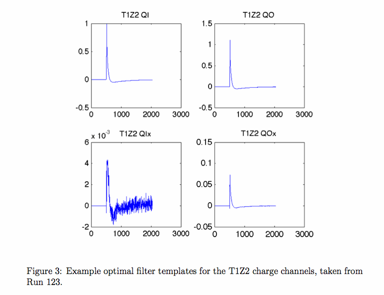
Figure 1: Example optimal filter templates for the T1Z2 charge channels, taken from Run 123.

The usual optimal filter minimizes $<code>\chi^{2}</code>$ in the frequency domain for the following equation:

S = aA + n

The algorithm returns a single amplitude estimate $<code>\hat{a}</code>$ given a template $<code>A(t)</code>$ , signal $<code>S(t)</code>$ , and noise spectrum $<code>n(f)</code>$ . In our case we generalize the optimal filter to reconstruct two amplitudes $<code>a_{I}</code>$ and $<code>a_{O}</code>$ simultaneously, given these four templates and two noise spectra, $<code>n_{O}</code>$ and $<code>n_{I}</code>$ . The equation to be solved now takes the form of a matrix expression:

\begin{pmatrix}
S_{I}\\
S_{O}
\end{pmatrix}
=
\begin{pmatrix}
A_{I} &A_{Ix} \\
A_{Ox} &A_{O}
\end{pmatrix}
\begin{pmatrix}
a_{I}\\
a_{O}
\end{pmatrix}
+
\begin{pmatrix}
n_{I}\\
n_{O}
\end{pmatrix}

We can rewrite this in essentially the form we’re used to, as long as we convert everything to vectors and matrices:

\vec{S}=\tilde{A}\cdot\vec{a}+\vec{n}

The entire OF analysis follows through. We can construct a $<code>\chi^{2}</code>$ function in frequency space just as before. Note that this $<code>\chi^{2}</code>$ has the number of degrees of freedom appropriate to 2 traces, rather than 1. This is why QSOFchisq peaks around 4096 for Soudan data while a single trace has 2048 samples.

\chi^{2}(a_{I},a_{O})=\sum_{freq}\Big(\frac{|S_{I}-(a_{I}A_{I}+a_{O}A_{Ix})|^{2}}{n_{I}^{2}}+\frac{|S_{O}-(a_{I}A_{Ox}+a_{O}A_{O})|^{2}}{n_{O}^{2}}\Big)

We then demand that the derivatives of this $<code>\chi^{2}</code>$ function with respect to $<code>a_{I}</code>$ and $<code>a_{O}</code>$ vanish at the desired estimates $<code>\hat{a}_{I}</code>$ and $<code>\hat{a}_{O}</code>$ , giving the expression:

\begin{pmatrix}
\sum\Re\Big(\frac{\tilde{A}_{I}^{\ast}}{\tilde{n}_{I}^{2}}\tilde{S}_{I}+\frac{\tilde{A}_{Ox}^{\ast}}{\tilde{n}_{O}^{2}}\tilde{S}_{O}\Big)\\
\sum\Re\Big(\frac{\tilde{A}_{Ix}^{\ast}}{\tilde{n}_{I}^{2}}\tilde{S}_{I}+\frac{\tilde{A}_{O}^{\ast}}{\tilde{n}_{O}^{2}}\tilde{S}_{O}\Big)\end{pmatrix}
=
\begin{pmatrix}
\sum\frac{|\tilde{A}_{I}|^{2}}{\tilde{n}_{I}^{2}}+\frac{|\tilde{A}_{Ox}|^{2}}{\tilde{n}_{O}^{2}} &\sum\Re\Big(\frac{\tilde{A}_{I}^{\ast}\tilde{A}_{Ix}}{\tilde{n}_{I}^{2}}+\frac{\tilde{A}_{O}^{\ast}\tilde{A}_{Ox}}{\tilde{n}_{O}^{2}} \\
\sum\Re\Big(\frac{\tilde{A}_{I}^{\ast}\tilde{A}_{Ix}}{\tilde{n}_{I}^{2}}+\frac{\tilde{A}_{O}^{\ast}\tilde{A}_{Ox}}{\tilde{n}_{O}^{2}} &\sum\frac{|\tilde{A}_{O}|^{2}}{\tilde{n}_{O}^{2}}+\frac{|\tilde{A}_{Ix}|^{2}}{\tilde{n}_{I}^{2}}
\end{pmatrix}
\begin{pmatrix}
a_{I}\\
a_{O}
\end{pmatrix}

If we write the central matrix as $<code>T_{Q}</code>$ , the solution is formally given by:

\begin{pmatrix}
a_{I}\\
a_{O}
\end{pmatrix}
=
T_{Q}^{-1}\begin{pmatrix}
\sum\Re\Big(\frac{\tilde{A}_{I}^{\ast}}{\tilde{n}_{I}^{2}}\tilde{S}_{I}+\frac{\tilde{A}_{Ox}^{\ast}}{\tilde{n}_{O}^{2}}\tilde{S}_{O}\Big)\\
\sum\Re\Big(\frac{\tilde{A}_{Ix}^{\ast}}{\tilde{n}_{I}^{2}}\tilde{S}_{I}+\frac{\tilde{A}_{O}^{\ast}}{\tilde{n}_{O}^{2}}\tilde{S}_{O}\Big)\end{pmatrix}

Note that most of the laborious computation in this last expression only needs to be performed once, rather than every time we process a trace. The optimal filter file stores the 2 X 2 matrix $<code>T_{Q}^{-1}</code>$ , as well as the various filters used on the right hand side:

\frac{\tilde{A}_{I}^{\ast}}{\tilde{n}_{I}^{2}},\frac{\tilde{A}_{O}^{\ast}}{\tilde{n}_{O}^{2}},
\frac{\tilde{A}_{Ix}^{\ast}}{\tilde{n}_{I}^{2}},
\frac{\tilde{A}_{Ox}^{\ast}}{\tilde{n}_{O}^{2}}

The two-channel ionization optimal filter is thus equivalent to four single-channel optimal filter operations, a couple of vector additions, and a single matrix multiplication.

Start time of pulse¶

Implicit in the above calculation is that a start time (delay) for the charge pulses is already determined, which is not the case in reality. Ideally we would repeat the above operation for a variety of start times and choose the fit with the best start time by some measure (such as the time that gives the minimum chisq). Unfortunately, this operation is very slow and it is not obvious how to accelerate it with iFFTs. Currently there are two options for finding the start time in BatRoot. One is a fast algorithm adopted from Darkpipe, the other is a slow algorithm but gives a more accurate start time on average for pulses with low signal to noise.

In the fast algorithm option, BatRoot computes the time offset using the sum of the two traces and then just applies this offset for a single matrix computation. This offset is chosen by finding the delay that yields the largested summed amplitude when the optimal filter is applied individually to the Qinner and Qouter pulses (without cross talk components). Then the full cross talk calculation is performed with this delay. Note that there are possible ambiguities if the two ionization pulses ever have opposite signs, e.g. in the so-called “ear” of a qi-versus-qo plot.

In the slow algorithm option, BatRoot performs the cross-talk fit for each delay within a range of delays about the expected start time of the pulse. It then assigns the delay and fit results to the fit that has the smallest chisq in this range. This is the so called “chisq-minimization” routine. It may be turned on and off through the user analysis settings file. In order to keep the processing time from ballooning, the full chisq routine is only performed on pulses that exceed a user-defined threshold on the charge channels AND for all random triggers. The threshold is channel-specific. If it is set to the BatRoot default value of -999999, the chisq minimization is not performed and the delay is chosen based on the faster “maximum amplitude” routine.

Improvements from Sub-bin interpolation¶

The ionization optimal filter $<code>\chi^{2}</code>$ distribution forms a narrow band near 4096 at low energies, just as we expect. It has a tendency to curve upward slightly and widen substantially at higher energies, however. A slight upward curvature is expected because the ionization templates do not have infinite signal to noise - imperfections in the template push $<code>\chi^{2}</code>$ upward at high amplitudes. In older datasets (those produced before 2010), the more worrisome widening of the distribution at higher energies (which reduces the power of our pileup rejection) is due to the single-bin ( $<code>0.8\mu s</code>$ ) accuracy of our start time determination - for large pulses, even a difference in start time of a few hundred nanoseconds can appreciably increase $<code>\chi^{2}</code>$ . The latter effect has been ameliorated using a sub-bin interpolation of start time, amplitude and $<code>\chi^{2}</code>$ . Jeff Filippini originally demonstrated this for Berkeley calibration data in DarkPipe. A routine that is build off the full chisq minimization routine has since been implemented in BatRoot. Further discussion of this may be found in ebook notes 123Note41, 130Note28 and TFNote16. The figure below shows this widening of the chisq distribution without sub-bin interpolation:

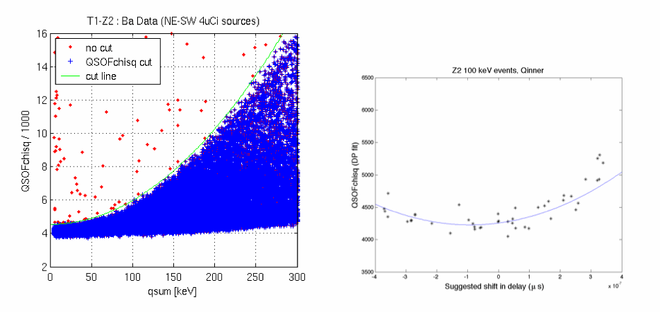
Figure 2: Left: QSOFchisq versus energy, showing widening at higher energies. Right: DarkPipe QSOFchisq values versus fitted sub-bin start time shifts for Qinner events in T1Z2 at ∼ 100 keV. This shows that a significant range of $<code>\chi^{2}</code>$ values can come from the same pulse with tiny shifts in start time. Note that the x-axis should be labeled in seconds rather than microseconds. The blue line shows a quadratic fit to events within $<code>0.4\mu s</code>$ of the apparent center. The curvature of the fit matches theory fairly well, though the offset and wings are less perfectly characterized.

Possible Extensions/Improvements¶

The time-saving threshold treatment of the chisq minimization routine is not ideal because it treats the lowest energy events differently from events above its threshold. Development of a new "N-Dimensional" optimal filter will allow us to circumvent this problem. This generalized routine will solve for the delay with the minimum chisq for events of all energies, while maintaining fast processing times.

References¶

Back to Top