Tutorial on Internet Monitoring & PingER at SLACTranslation into: Arabic (hosted by CouponToaster), Belorussian (hosted by Websitehostingrating), Hindi (hosted by Dealsdaddy), Indonesian (hosted by ChameleonJohn), Irish, Romanian (translated by EWSTranslate), Russian, Sindhi (hosted by Blog home), Spanish (translated by TheWordPoint), Ukrainian (translated by WriteMyPaperHub), Urdu (hosted by blog home), Les Cottrell, Warren Matthews and Connie Logg, Created January 1996; last Update: December 1st, 2014. |
Work partially funded by a DOE/MICS Field Work Grant for Internet End-to-end Performance Monitoring (IEPM).
The set of remote hosts to ping is provided by a file called pinger.xml (for more on this see the pinger2.pl documentation). This file consists of two parts: Beacon hosts which are automatically pulled daily from SLAC and are monitored by all MPs; other hosts which are of particular interest to the administrator of the MP. The Beacon hosts (and the particular hosts monitored by the SLAC MP) are kept in an Oracle database containing their name, IP address, site, nickname, location, contact etc. The Beacon list (and list of particular hosts for SLAC) and a copy of the database, in a format to simplify Perl access for analysis scripts, are automatically generated from the database on a daily basis.
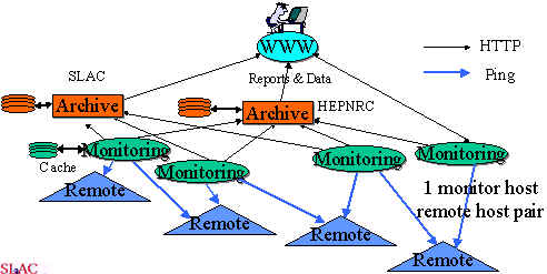
The archive sites gather the information, by using HTTP, from the monitor sites at regular intervals and archive it. They provide the archived data to the analysis site(s), that in turn provide reports that are available via the Web.
The PingER architecture is illustrated below:
We have also observed various pathologies with various remote sites when using ping. These are documented in PingER Measurement Pathologies.
The calibration and context in which the round trip metrics are measured are documented in PingER Calibration and Context, and some examples of how ping results look when taken with high statistics, and how they relate to routing, can be found in High statistics ping results.
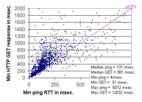
The remarkably clear lower boundary seen around y = 2x
is not surprising since:
a slope of 2 corresponds to HTTP GETs that take twice the ping
time; the minimum ping time is approximately the round trip time; and
a minimal TCP transaction involves two round trips, one round trip to exchange
the second to send the request and receive the response. The connection
termination is done asynchronously and so does not show up in the timing.
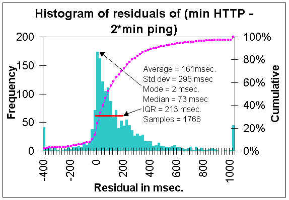
The lower boundary can also be visualized by displaying the distribution of residuals
between the measurements and the line y = 2 x(where y =
HTTP GET response time and x =
Minimum ping response time). Such a distribution is shown below. The steep in crease in
the frequency of measurements as one approaches zero residual value
(y=2x) is apparent.
The Inter Quartile Range (IQR), the residual range between where
25% and 75% of the
measurements fall, is about 220 msec, and is indicated on the plot by the
red line.
An alternate way of demonstrating that ping is related to Web performance is to show that ping can be used to predict which of a set of replicated Web servers to get a Web page from. For more on this see Dynamic Server Selection in the Internet, by Mark E. Crovella and Robert L. Carter.
The Firehunter Case Study of the Whitehouse Web Server showed that though ping response does not track abnormal Web performance well, in this case ping packet loss did a much better job.
The Internet quality of service assessment by Christian Huitema, provides measurements of the various components that contribute to web response. These components include: RTT, transmission speed, DNS delay, connection delay, server delay, transmission delay. It shows that the delays between sending the GET URL command and the reception of the first byte of the reponse is an estimate of server delay ("in many servers, though not necessarily all, this delay corresponds to the time needed to schedule the page requests, prepare the page in memory, and start sending data") and represents between 30 and 40% of the duration of the average transaction. To ease that, you probably need more powerful servers. Getting faster connections would obviously help the other 60% of the delay.
Also see the section below on Non Ping based tools for some correlations of throughput with round trip time and packet loss.
With measured data we are able to create long term baselines for expectations on means/medians and variability for response time, throughput, and packet loss. With these baselines in place we can set expectation, provide planning information, make extrapolations and look for exceptions (e.g. today's response time is more than 3 standard deviations greater than the average for the last 50 working days) and raise alerts.
We also use more complex tools such as FTP (to measure bulk transfer rates) and traceroute (to measure paths and number of hops). However, besides being more difficult to set up and automate, FTP is more intrusive on the network and more dependent on end node loading. Thus we use FTP mainly in a manual mode and to get an idea of how well the ping tests work (e.g. Correlations between FTP and Ping and Correlations between FTP throughput, Hops & Packet Loss). We have also compared PingER predictions of throughput with NetPerf measurements. Another way to correlate throughput measurements with packet loss is by Modeling TCP Throughput.
There are three factors that significantly impact call quality: latency, packet loss, jitter. Other factors include the codec type, the phone (analog vs. digital), the PBX etc.) We show how we calculate jitter later in this tutorial. Most tool-based solutions calculate what is called an "R" value and then apply a formula to convert that to an MOS score. We do the same. This R to MOS calculation is relatively standard (see for example ITU - Telecommunication Standardization Sector Temporary Document XX-E WP 2/12 for a new method). The R value score is from 0 to 100, where a higher number is better. Typical R to MOS values are: R=90-100 => MOS=4.3-5.0 (very satisfied), R=80-90=>MOS=4.0-4.3 (satisfied), R=70-80=>MOS=3.6-4.0 (some disatisfaction), R=60-70=>MOS=3.1-3.6 (more disatisfaction), R=50-60=>MOS=2.6-3.1 (Most disatisfaction), R=0-50=>MOS=1.0-2.6 (not recommended). To convert latency, loss, jitter to MOS we follow Nessoft's method. They use (in pseudo code):
#Take the average round trip latency (in milliseconds), add
#round trip jitter, but double the impact to latency
#then add 10 for protocol latencies (in milliseconds).
EffectiveLatency = ( AverageLatency + Jitter * 2 + 10 )
#Implement a basic curve - deduct 4 for the R value at 160ms of latency
#(round trip).  Anything over that gets a much more agressive deduction.

if EffectiveLatency < 160 then
   R = 93.2 - (EffectiveLatency / 40)
else
   R = 93.2 - (EffectiveLatency - 120) / 10

#Now, let us deduct 2.5 R values per percentage of packet loss (i.e. a
#loss of 5% will be entered as 5).
R = R - (PacketLoss * 2.5)

#Convert the R into an MOS value.(this is a known formula)
if R < 0 then
   MOS = 1
else
   MOS = 1 + (0.035) * R + (.000007) * R * (R-60) * (100-R)
Also see the following for some measurement tools and/or explanations:
An improved form of the above equation can be found in: Modeling TCP throughput: A simple model and its empirical validation by J. Padhye, V. Firoiu, D. Townsley and J. Kurose, in Proc. SIGCOMM Symp. Communications Architectures and Protocols Aug. 1998, pp. 304-314.
Rate=min(Wmax/RTT, 1/((RTT/sqrt(2*b*p/3)+min(1, 3*sqrt(3*b*p/8))*(1+32*p*p))))
where:The behavior of throughput as a function of loss and RTT can be seen by looking at Throughput versus RTT and loss. We have used the formula Mathis to compare PingER and NetPerf measurements of throughput.
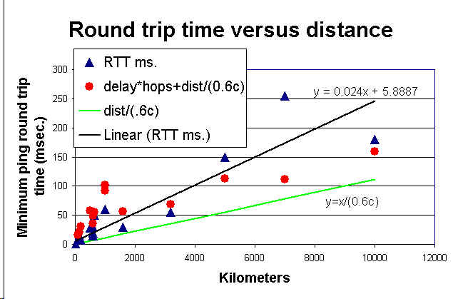
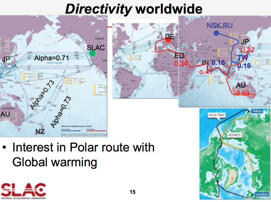
RTD=Round Trip Distance,
RTD[km] = Directivity * min_RTT[msec] * 200 [km/msec]
Directivity allows for delays in network equipment and
indirectness of the actual route.
D = 1 way distance
Directivity = D(km) / (min_RTT[msec] * 100 [km/msec])
 |
By plotting a 3D plot of node versus time versus response we can look for correlations of several nodes having poor performance or being unreachable at the same time (maybe due to a common cause), or a given node having poor response or being unreachable for an extended time. To the left is an example showing several hosts (in black) all being unreachable around 12 noon. |
| Tables of monthly medians of the prime time (7am- 7pm weekday) 1000 byte ping response time and 100 byte ping packet loss allow us to view the data going back for longer periods. This tabular data can be exported to Excel and charts made of the long term ping packet loss performance. | 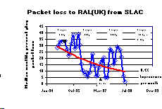 |
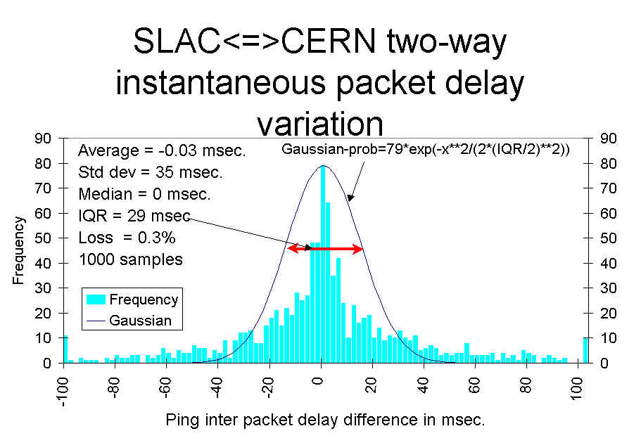
One method requires injecting packets at regular intervals into the network and measuring the variability in the arrival time. The IETF has IP Packet Delay Variation Metric for IP Performance Metrics (IPPM) (see also RTP: A Transport Protocol for Real-Time Applications, RFC 2679 and RFC 5481
We measure the instantaneous variability or "jitter" in two ways.
By viewing the Ping "jitter" between SLAC and CERN, DESY & FNAL it can be seen that the two methods of calculating jitter track one another well (the first method is labelled IQR and the second labelled IPD in the figure). They vary by two orders of magntitude over the day. The jitter between SLAC & FNAL is much lower than between SLAC and DESY or CERN. It is also noteworthy that CERN has greater jitter during the European daytime while DESY has greater jitter during the U.S. daytime.
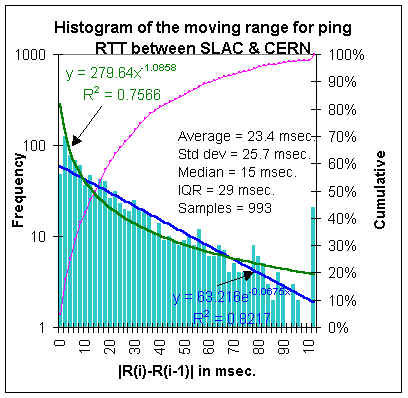
We have also obtained a measure of the jitter by taking the absolute value dR, i.e. |dR|. This is sometimes referred to as the "moving range method" (see Statistical Design and Analysis of Experiments, Robert L. Mason, Richard F. Guest and James L. Hess. John Wiley & Sons, 1989). It is also used in RFC 2598 as the definition of jitter (RFC 1889 has another definition of jitter for real time use and calculation) See the Histogram of the moving range for an example. In this figure, the magenta line is the cumulative total, the blue line is an exponentail fit to the data, and the green line is a power series fit to the data. Note that all 3 of the charts in this section on jitter are representations of identical data.
 In order to more closely understand the requirements for VoIP and in particular
the impacts of applying Quality of Service (QoS) measures, we have set up
a VoIP testbed between SLAC and LBNL. A rough schematic is shown to the right.
Only the SLAC half circuit is shown in the schematic, the LBNL end is similar.
A user can lift the phone connected to the PBX at the SLAC end and
call another user on a phone at LBNL via the VoIP Cisco router gateway.
The gateway encodes, compresses etc. the voice stream into IP packets (using the
G.729 standard)
creating roughly 24kbps of traffic. The VoIP stream include both TCP (for signalling)
and UDP packets. The
connection from the ESnet router to the ATM cloud is a 3.5 Mbps ATM permanent
virtual circuit (PVC).
With no competing traffic on the link, the call connects and the conversation
proceeds normally with good quality. Then we inject 4 Mbps of traffic onto
the shared 10 Mbps Ethernet that the VoIP router is connected to. At this stage,
the VoIP connection is broken and no further connections can be made. We then
used the Edge router's Committed Access Rate (CAR) feature to label the VoIP
packets' by setting Per Hop Behavior (PHB) bits. The ESnet router is then
set to use the
Weighted Fair Queuing (WFQ) feature to expedite the VoIP packets.
In this setup voice connections can again be made and the conversation
is again of good quality.
In order to more closely understand the requirements for VoIP and in particular
the impacts of applying Quality of Service (QoS) measures, we have set up
a VoIP testbed between SLAC and LBNL. A rough schematic is shown to the right.
Only the SLAC half circuit is shown in the schematic, the LBNL end is similar.
A user can lift the phone connected to the PBX at the SLAC end and
call another user on a phone at LBNL via the VoIP Cisco router gateway.
The gateway encodes, compresses etc. the voice stream into IP packets (using the
G.729 standard)
creating roughly 24kbps of traffic. The VoIP stream include both TCP (for signalling)
and UDP packets. The
connection from the ESnet router to the ATM cloud is a 3.5 Mbps ATM permanent
virtual circuit (PVC).
With no competing traffic on the link, the call connects and the conversation
proceeds normally with good quality. Then we inject 4 Mbps of traffic onto
the shared 10 Mbps Ethernet that the VoIP router is connected to. At this stage,
the VoIP connection is broken and no further connections can be made. We then
used the Edge router's Committed Access Rate (CAR) feature to label the VoIP
packets' by setting Per Hop Behavior (PHB) bits. The ESnet router is then
set to use the
Weighted Fair Queuing (WFQ) feature to expedite the VoIP packets.
In this setup voice connections can again be made and the conversation
is again of good quality.
| Date | All Hosts | ESnet | N. America | International |
|---|---|---|---|---|
| Jul '95 |  |
 |
 |
 |
| Mar '96 |  |
 |
 |
 |
One can also measure the frequency of outage lengths using active probes and noting the time duration for which sequential probes do not get through.
Ano/ther metric that is sometimes used to indicate the availability of a phone circuit is Error-free seconds. Some measurements on this can be found in Error free seconds between SLAC, FNAL, CMU and CERN.
There is also an IETF RFC on Measuring Connectivity and a document on A Modern Taxonomy of High Availability which may be useful.
In the above plot, the loss and response time are measured during SLAC prime time (7am - 7pm, weekdays), the other measures are for all the time.
| 0-0.4s | High productivity interactive response |
| 0.4-2s | Fully interactive regime |
| 2-12s | Sporadically interactive regime |
| 12s-600s | Break in contact regime |
| 600s | Batch regime |
There is a threshold around 4-5s where complaints increase rapidly. For some newer Internet applications there are other thresholds, for example for voice a threshold for one way delay appears at about 150ms (see ITU Recommendation G.114 One-way transmission time, Feb 1996) - below this one can have toll quality calls, and above that point, the delay causes difficulty for people trying to have a conversation and frustration grows.
For keeping time in music, Stanford researchers found that the optimum amount of latency is 11 milliseconds. Below that delay and people tended to speed up. Above that delay and they tend to slow down. After about 50 millisecond (or 70), performances tended to completely fall apart.
The human ear perceives sounds as simultaneous only if they are heard within 20 ms of each other, see http://www.mercurynews.com/News/ci_27039996/Music-at-the-speed-of-light-is-researchers-goal
For real-time multimedia (H.323) Performance Measurement and Analysis of H.323 Traffic gives one way delay (roughly a factor two to get RTT), of: 0-150ms = Good, 150-300ms=Accceptable, and > 300ms = poor.
The SLA for one-way network latency target for Cisco TelePresence is below 150 msec. This does not include latency induced by encoding and decoding at the CTS endpoints.
All packets that comprise a frame of video must be delivered to the TelePresence end point before the replay buffer is depleted. Otherwise degradation of the video quality can occur. The peak-to-peak jitter target for Cisco TelePresence is under 10 msec.
The paper on The Internet at the Speed of Light gives several examples of the importance of reducing the RTT. Examples include search engines such as Google and Bing, Amazon sales and the stock exchange
For real time haptic control and feedback for medical operations, Stanford researchers (see Shah, A., Harris, D., & Gutierrez, D. (2002). "Performance of Remote Anatomy and Surgical Training Applications Under Varied Network Conditions." World Conference on Educational Multimedia, Hypermedia and Telecommunications 2002(1), 662-667 ) found that a one way delay of <=80msec. was needed.
The Internet Weather map identifies as bad any links with delays over 300ms.
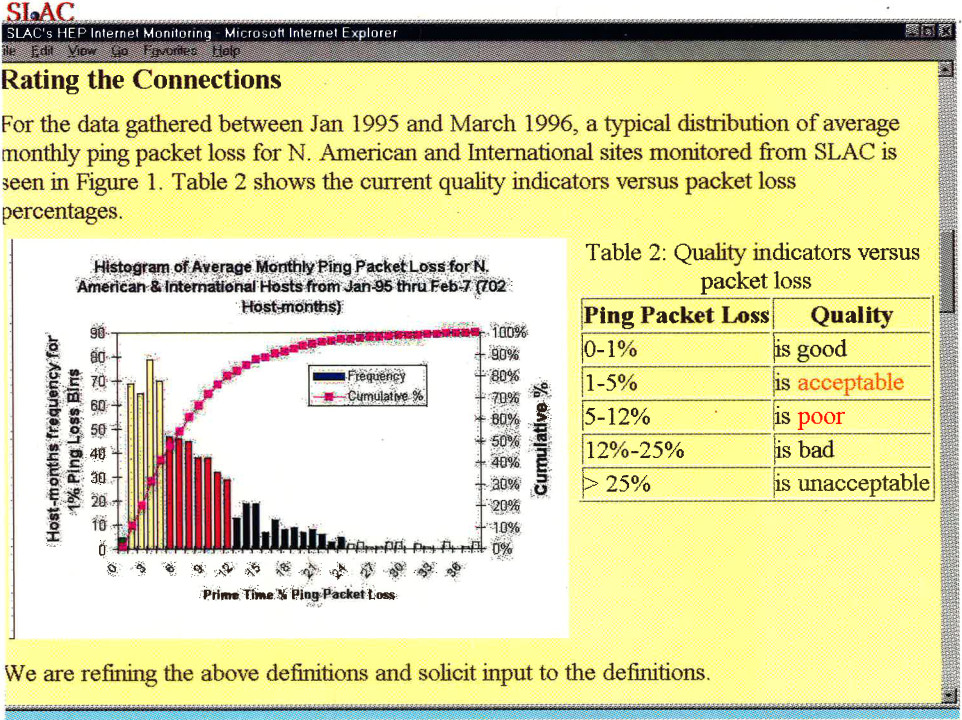
Originally the quality levels for packet loss were set at 0-1% = good, 1-5% =
acceptable, 5-12% = poor, and greater than 12% = bad.
More recently,
we have refined the levels to 0-0.1% excellent, 0.1-1% = good, 1-2.5% = acceptable, 2.5-5% =
poor, 5%-12% = very poor, and greater than 12% = bad.
Changing the thresholds reflects changes in our emphasis, i.e. in 1995
we were primarily be concerned with email and ftp. This
quote from Vern Paxson sums up the main concern at the time:
Conventional wisdom among TCP researchers holds that a loss
rate of 5% has a significant adverse effect on TCP performance,
because it will greatly limit the size of the congestion
window and hence the transfer rate, while 3% is often
substantially less serious.
In other words, the complex behaviour of the Internet results
in a significant change when packet loss climbs above 3%.
In 2000 we were
also concerned with X-window applications, web performance, and packet video
conferencing. By 2005 we were interested in the real-time requirements of VoIP
and are starting to look at voice over IP.
As a rule, packet loss in VoIP (and VoFi) should never exceed 1 percent, which essentially means one voice skip every three minutes. DSP algorithms may compensate for up to 30 ms of missing data; any more than this, and missing audio will be noticeable to listeners.
The Automotive Network eXchange (ANX) sets
the threshold for packet loss rate (see
ANX /
Auto Linx Metrics) to be less than 0.1%.
The ITU TIPHON working group (see General aspects of Quality of Service (QOS), DTR/TIPHON-05001 V1.2.5 (1998-09) technical Report) has also defined < 3% packet loss as being good, > 15% for medium degradation, and 25% for poor degradation, for Internet telephony. It is very hard to give a single value below which packet loss gives satisfactory/acceptable/good quality interactive voice. There are many other variables involved including: delay, jitter, Packet Loss Concealment (PLC), whether the losses are random or bursty, the compression algorithm (heavier compression uses less bandwidth but there is more sensitivity to packet loss since more data is contained/lost in a single packet). See for example Report of 1st ETSI VoIP Speech Quality Test Event, March 21-18, 2001, or Speech Processing, Transmission and Quality Aspects (STQ); Anonymous Test Report from 2nd Speech Quality Test Event 2002 ETSI TR 102 251 v1.1.1 (2003-10) or ETSI 3rd Speech Quality Test Event Summary report, Conversational Speech Quality for VoIP Gateways and IP Telephony.
Jonathan Rosenberg of Lucent Technology and Columbia University in G.729 Error Recovery for Internet Telephony presented at the V.O.N. Conference 9/1997 gave the following table showing the relation between the Mean Opinion Score (MOS) and consecutive packets lost.
| Consecutive frames lost | 1 | 2 | 3 | 4 | 5 |
|---|---|---|---|---|---|
| M.O.S. | 4.2 | 3.2 | 2.4 | 2.1 | 1.7 |
| Rating | Speech Quality | Level of distortion |
|---|---|---|
| 5 | Excellent | Imperceptible |
| 4 | Good | Just perceptible, not annoying |
| 3 | Fair | Perceptible, slightly annoying |
| 2 | Poor | Annoying but not objectionale |
| 1 | Unsatisfactory | Very annoying, objectionable |
So we set "Acceptable" packet loss at < 2.5%. The paper Performance Measurement and Analysis of H.323 traffic gives the following for VoIP (H.323): Loss = 0%-0.5% Good, = 0.5%-1.5% Acceptable and > 1.5% = Poor.
The above thresholds assumes a flat random packet loss distribution. However, often the losses come in bursts. In order to quantify consecutive packet loss we have used, among other things, the Conditional Loss Probability (CLP) defined in Characterizing End-to-end Packet Delay and Loss in the Internet by J. Bolot in the Journal of High-Speed Networks, vol 2, no. 3 pp 305-323 December 1993 (it is also available on the web). Basically the CLP is the probablility that if one packet is lost the following packet is also lost. More formally Conditional_loss_probability = Probability(loss(packet n+1)=true | loss(packet n) = true). The causes of such bursts include the convergence time required after a routing change (10s to 100s of seconds), loss and recovery of sync in DSL network (10-20 seconds), and bridge spanning tree re-configurations (~30 seconds). More on the impact of of bursty packet loss can be found in Speech Quality Impact of Random vs. Bursty Packet losses by C. Dvorak, internal ITU-T document. This paper shows that whereas for random loss the drop off in MOS is linear with % packet loss, for bursty losses the fall off is much faster. Also see Packet Loss Burstiness. The drop off in MOS is from 5 to 3.25 for a change in packet loss from 0 to 1% and then it is linear falling off to an MOS of about 2.5 by a loss of 5%.
Other monitoring efforts may choose different thresholds possibly because they are concerned with different applications. MCI's traffic page labelled links as green if they have packet loss < 5%, red if > 10% and orange in between. The Internet Weather Report we colored < 6% loss as green and > 12% as red, and orange otherwise. So they are both more forgiving than we or or at least have less granularity. Gary Norton in Network World Dec. 2000 (p 40), says "If more than 98% of the packets are delivered, the users should experience only slightly degraded response time, and sessions should not time out".
The figure below shows the frequency distributions for the average
monthly packet loss for about 70 sites seen from SLAC between January 1995 and
November 1997.
Due to the high amount of compression and motion-compensated prediction utilized by TelePresence video codecs, even a small amount of packet loss can result in visible degradation of the video quality. The SLA for packet loss target for Cisco TelePresence should be below 0.05 percent on the network.
For real time haptic control and feedback for medical operations, Stanford researchers found that loss was not a critical factor and losses up to 10% could be tolerated.
However for high performance data throughput over long distances (high RTTs), as can be seen in ESnet's article on Packet Loss, losses of as little as 0.0046% (1 packet loss in 22,000) on 10Gbps links with the MTU set at 9000Bytes (the impact is greater with default MTU's of 1500Bytes) result in factors of 10 reduction in throughput for RTTs > 10msec.
| Degradation category | Peak jitter |
|---|---|
| Perfect | 0 msec. |
| Good | 75 msec. |
| Medium | 125 msec. |
| Poor | 225 msec. |
Web browsing and mail are fairly resistent to jitter, but any kind of streaming media (voice, video, music) is quite suceptible to Jitter. Jitter is a symptom that there is congestion, or not enough bandwidth to handle the traffic.
The jitter specifies the length of the VoIP codec playout buffers to prevent over- or under-flow. An objective could be to specify that say 95% of packet delay variations should be within the interval [-30msec, +30msec].
For real-time multimedia (H.323) Performance Measurement and Analysis of H.323 Traffic gives for one way: jitter = 0-20ms = Good, jitter = 20-50ms = acceptable, > 50ms = poor. We measure round-trip jitter which is roughly two times the one way jitter.
For real time haptic control and feedback for medical operations, Stanford researchers found that jitter was critical and jitters of < 1msec were needed.
"Queuing theory suggests that the variation in round trip time, o, varies proportional to 1/(1-L) where L is the current network load, 0<=L<=1. If an Internet is running at 50% capacity, we expect the round trip delay to vary by a factor of +-2o, or 4. When the load reaches 80%, we expect a variation of 10." Internetworking with TCP/IP, Principle, Protocols and Architecture, Douglas Comer, Prentice Hall. This suggests one may be able to get a measure of the utilization by looking at the variability in the RTT. We have not validated this suggestion at this time.
The Bellcore Generic Requirement 929 (GR-929-CORE Reliability and Quality Measurements for Telecommunications Systems (RQMS) (Wireline), is actively used by suppliers and service providers as the basis of supplier reporting of quarterly performance measured against objectives. Each year, following publication of the most recent issue of GR-929-CORE, such revised performance objectives are implemented) indicates that the the core of the phone network aims for a 99.999% availability, That translates to less than 5.3 minutes of downtime per year. As written the measurement does not include outages of less than 30 seconds. This is aimed at the current PSTN digital switches (such as Electronic Switching System 5 (5ESS) and the Nortel DMS250), using todays voice-over-ATM technology. A public switching system is required to limit the total outage time during a 40-year period to less than two hours, or less than three minutes per year, a number equivalent to an availability of 99.99943%. With the convergence of data and voice, this means that data networks that will carry multiple services including voice must start from similar or better availability or end-users will be annoyed and frustrated.
Levels of availability are often cast into a Service Level Agreements. The table below (based on Cahners In-Stat survey of a sample of Application Service Providers (ASPs)) shows the levels of availability offered by ASPs and the levels chosen by customers.
| Levels offered | Chosen by customer | |
|---|---|---|
| Less than 99% | 26% | 19% |
| 99% availability | 39% | 24% |
| 99.9% availability | 24% | 15% |
| 99.99% availability | 15% | 5% |
| 99.999% availability | 18% | 5% |
| More than 99.999% availability | 13% | 15% |
| Don't know | 13% | 18% |
| Weighted average of availability offered | 99.5% | 99.4% |
At the same time it is critical to choose the remote sites and host-pairs
carefully so that they are representative of the information one is hoping to
find out. We have therefore selected a set of about 50 "Beacon Sites" which
are monitored by all monitoring sites and which are representative of the various
affinity groups we are interested in.
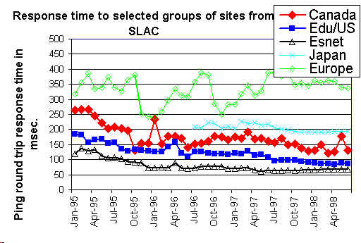
An example of a graph showing ping response times for groups of sites is seen
below:
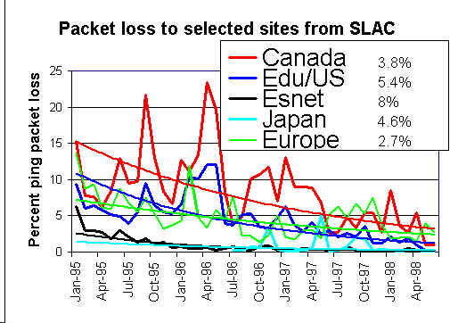
The percentages shown to the right of the legend of the packet lost chart are
the improvements (reduction in packet loss) per month for exponential trend
line fits to the packet loss data. Note that a 5%/month improvement is equivalent to
44%/year improvement (e.g. a 10% loss would drop to 5.6% in a year).
RIPE also has a Test Traffic project to make independent measurements of connectivity parameters, such as delays and routing-vectors in the Internet. A RIPE host is installed at SLAC.
The NLANR Active Measurement Program (AMP) for HPC awardees is intended to improve the understanding of how high performance networks perform as seen by participating sites and users, and to help in problem diagnosis for both the network's users and its providers. They install a rack mountable FreeBSD machine at sites and make full mesh active ping measurements between their machines, with the pings being launched at about 1 minute intervals. An AMP machine is installed at SLAC.
More detailed comparisons of Surveyor, RIPE, PingER and AMP can be found at Comparison of some Internet Active End-to-end Performance Measurement projects.
SLAC is also a NIMI (National Internet Measurement Infrastructure) site. This project may be regarded as complementary to the Surveyor project, in that it (NIMI) is more focussed on providing the infrastructure to support many measurement methodologies such as one way pings, TReno, traceroute, PingER etc.
Waikato University in New Zealand is also deploying Linux hosts each with a GPS receiver and making one way delay measurements. For more on this see Waikato's Delay Findings page. Unlike the AMP, RIPE and Surveyor projects, the Waikato project makes passive measurements, of the normal traffic between existing pairs, using CRC based packet signatures to identify packets recorded at the 2 ends.
The sting TCP-based network measurement tool is able to actively measure the packet loss in both the forward and reverse paths between pairs of hosts. It has the advantage of not requiring a GPS, and not being subject to ICMP rate limiting or blocking (according to an ISI study ~61% of the hosts in the Internet do not repond to pings), however it does require a small kernel modification.
If the one way delay (D) is known for both directions of an
Internet pair of nodes (a,b),
then the round trip delay R can be calculated as follows:
R = Da=>b + Db=>a
where Da=>b is the one way delay measured from node a to node
b and vice versa.
The two way packet loss P can be derived from the one way losses (p)
as follows:
P = pa=>b + pb=>a - pa=>b *
pb=>a
where pa=>b is the one way packet loss from node a to
b and vice versa.
John MacAllister at Oxford developed Traceping Route Monitoring Statistics based on the standard traceroute and ping utilities. Statistics were gathered at regular intervals for 24-hour periods and provided information on routing configuration, route quality and route stability.
TRIUMF also has a very nice Traceroute Map tool that shows a map of the routes from TRIUMF to many other sites. We are looking at providing a simplification of such maps to use the Autonomous Systems (AS) passed through rather than the routers.
One can also plot the FTP throughput versus traceroute hop count as well as ping response and packet loss to look for correlations.
Many sites are appearing that run traceroute servers (the source code (in Perl) is available) which help in debugging and in understanding the topology of the Internet.
Some sites provide access to network utilities such as nslookup to allow one to find out more about a particular node. A couple of examples are SLAC and TRIUMF.
 [
Feedback |
Reporting Problems
]
[
Feedback |
Reporting Problems
]