Back to Agenda
In this third hands-on you will learn:
$ cd <tutorial> #change <tutorial> to your working directory |
Follow the instructions of Hands On
1 to configure with cmake the example and build it.
Try out the application:
$ source <where-G4-was-installed>/bin/geant4.[c]sh |
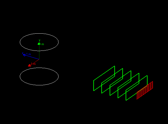
This geometry should be displayed if you have visualization
enabled:
The geomtry is basically the same as in Hands On 2, we will start from here to build a spectrometer. The first arm is already defined, and in the first exercise you will build the second arm and a calorimetric system:
The second arm is movable and can be rotated, between runs. The magnetic-field can also be set to user value.
At the end of this hands on part the complete geometry will look
like:

Different aspects of the geometry will be covered in this
exercise. There are 6 steps involved in this exercise. Depending on
how you build the geometry it is guaranteed that the
application will compile and work correctly only when the first 5
steps are concluded (however it is a good idea to try to compile at
each step to check for typos and errors).
The last step is optional because it has the goal
to change visualization attributes (it make sense only if you have
visualization enabled).
Different aspects of defining geometry will be presented:
G4PVPlacement (these have been already covered in Hands On 2).G4PVParametrised to place multiple copies of
the same volume with dimensions/position parametrised by the copy
number.
Check the DetectorConstruction.hh file, since many
variables you will need are already defined there.
Implement the second hodoscope.
The second hodoscope is composed on 25 planes of dimensions: 10x40x1 cm. The hodoscopes tiles are composed of scintillator material. Instantiate a single shape and logical volume. Place 25 physical volume placements in the second arm mother volume. Each tile is positioned at Y=Z=0 with respect to the mother volume, while the X coordinates depends on the tile numnber.
Hint: Check what is done for the hodosope of the first arm. Remember dimensions passed to Geant4 shape classes are half the full dimention.
| DetectorConstruction File: |
// =============================================
|
Build the drift chambers.
The second arm contains 5 drift chambers made of argon gas with dimensions 300x60x2 cm. These are equally spaced inside the second arm at distances from -2.5 m to -0.5 m along the Z coordinate.
Hint: Use same methods used for step 1.
| DetectorConstruction File: |
// Step 2: Add 5 drift chambers made of argon, with dimensions (X,Y,Z):
|
Add a virtual wire plane in the drift chambers.
Add a plane of wires in the drift chambers of step 2. To simplify our problem we do not describe the single wires, instead we add a new argon-filled volume of dimensions 300x60x0.02 cm in the center of each of the five drift chambers.
This exercise is technically simple (a single placement), however it shows a very useful concept: we create a single instance of this volume and we place it once inside the mother logical volume (the drift chamber logical volume), since the mother volume is repeated with five placements, each of them gets its own wire plane. We are reducing the number of class instances needed for the description of our geometry (and thus reducing the memory footprint of our application, beside making the code compact and readable).
| DetectorConstruction File: |
// Step 3: Add a virtual wire plane of (300,60,0.02)cm
|
Build an electro-magnetic calorimeter.
An electro-magnetic calorimeter has the goal to measure the energy of an absorbed particle. Its dimensions are such that an electron or gamma of the tipical beam energy is fully absorbed (via an electro-magnetic shower) in the calorimeter (while hadrons, such as protons, only leave part of their energy in an electromagnetic calorimeter, because it is "too short"). In our example we implement a homogenous calorimeter made of a matrix of CsI crystals (a charged paricles emits light when interacting with this material, the quantity of light produced is proportional to the lost energy).
Build a 300x60x30 cm CsI caloriemter. The calorimeter is made of a
matrix of 15x15x30 cm crystals. Instead of using placements we show
how to use parametrised solids. The idea is that the position of the
placement is a function of the crystal number. The parametrisation
class is already available for you in
CellParametrisation. Study the method
CellParameterisation::ComputeTransformation(...) to
understand how the calorimeter cells are implemented.
The calorimeter should be places at 2 m downstream of the second arm
mother volume.
Hint: You can skip the cell definition and the application will work anyway with a single giant crystal. If you are running out of time, you can come back to parametrisations later.
| DetectorConstruction File: |
// Step 4: Build CsI EM-calorimeter of (300,60,30)cm
|
Implement the hadronic calorimeter
This is a sampling calorimeter made of lead as absorber material (used for its high density) interleaved with plates of scintillator (the active material). It is called sampling because only a fraction of the energy lost by the particles is measured (the one lost in the active material), however this is proportional to the total energy loss and hence to the impinging particle energy (you may be aware of the problems with non-compensation, but we will not discuss them here).
Implement the calorimeter using replicas to slice a volume. Each cell has 20 layers of 4 cm thick lead plate and 1 cm
thick scintillator plate. The size of the plate is 30 cm square. The
calorimeter array has 10 horizontal columns in 2 vertical rows. Here is a
schematic drawing of the calorimeter.

You can now test the setup, use UI commands
/tutorial/detector/armAngle,
/tutorial/field/value to move the second arm and set the
magnetic field. Note that geometry can be changed only between
runs. The methods DefineCommands gives an example on how
to define commands (however this is an advanced topic not discussed in
this Hands Ons). Use the
help UI command to get help on these commands.
| DetectorConstruction File: |
// Step 5: Add a "sandwich" hadronic calorimeter of dimensions:
|
Give visualization attributes to the second arm volumes.
Note that hadronic calorimeter sub-structure is made invisbile to reduce visual clutter. This is helpful to hide some less important details of the simulation.
| DetectorConstruction File: |
// visualization attributes ------------------------------------------------
|
In this exercise we will cover basic aspects of retrieving
physics quantities from the simulation kernel. The basic simulation output is a
hit (class G4VHit): an energy deposit in space and time. We are tipically not
interested in hits in all detector elements, but instead we want to
register this informaiton only for the relevant sensitive detector componets to
simulate the detector read-out (e.g. scintillator tiles from the hadronic
calorimeter, and not the lead absorber).
We will show how to measure a simulated quantity, for each event, for the hodoscopes. The goal is to measure at what time and in which tile there was a hit.
The exercise is divided in three parts, and you will have to modify four files:
HodoscopeHit.hh and HodoscopeHit.cc files that implement the hit
class for the hodoscope.HodoscopeSD.cc that implements the hodoscope sensitive
detector.DetectorConstruction.cc that instantiates the sensitive detector
and attaches it to the correct logical volume.Create a hit class.
You will need to modify the HodoscopeHit class. A skeleton is
already preapred, add two data members that identify which hodoscope
tile has fired and register the time of fire.
Note, to make the code
compile empty Constructor, operator new and delete have been
implemented. You should remove this empty implementation and
implement the correct methods. Implement/modify the Print method to dump on
screen hit content.
Important note on operator new and
delete: hits can put some
pressure on CPU, because, for each event, many hits may be created
be created (via a call to operator new) and deleted at the end of the
event. Allocating on the heap (via new/delete) is a
(relatively) CPU
intensive operation, thus the pure handling of hits may cause some
performance degradation in a complex application.
To mitigate this we
have an allocator that allows to efficently re-use memory and
avoid many calls to new/delete.
The first time a hit is created a memory pool is created that can hold
(like in an array) many instances of hits. Each time a hit is created
with new operator we first look in this pool for an available
pre-allocatd hit memory location. If a space is available, we
re-use this space, otherwise we grow the pool to contain more
hits.
With this technique we reduce substantially the allocation of memory
on the heap.
Note that an additional complication is that in multi-threading
environments special attention is needed for the creation of allocators.
We recognize this is quite technical and advanced topic. If you do not feel
confortable with this, you can remove from the HodoscopeHit.hh file
the lines defining the new and delete operators, the application will
work perfectly and since the hits are very simple and the simulation
program not so complex you will not see any CPU penalty.
This exercise implements a single sensitive detector and one hit type. In Hands On 4 additional sensitive detectors are used with hits in the drift chambers and in the calorimeters. You can study the code there to see additional types of hits (calorimeteric hits are of some interest since accumulate all energy deposits in a single cell).
| HodoscopeHit.hh file: |
class HodoscopeHit : public G4VHit
|
| Hodoscope.cc file: |
|
Create and manipulate hodoscope hits.
For this exercise you will modify HodoscopeSD.cc file. Some part of
the code is already implemented for you, in particular the
initialization of the hits collection. You need to modify the method
ProcessHits and implement the logic to extract time and
position.
Hint 1: Given a G4Step two points are defined
(G4StepPoint) that delimit the step itself. From each
point you can retrieve which volume the step belongs to via the
touchable history:
G4TouchableHistory* touchable = static_cast<G4TouchableHistory*>(
stepPoint->GetTouchable() );

G4int copyNumber = touchable->GetVolume()->GetCopyNo();
These two lines allows you to get the copy number of the volume
touched by the step (in our case the copy number for the hodoscope is
the tile number, see file DetectorConstruction.cc).
Hint 2: As we said there are two G4StepPoint
defining a G4Step, which one of the two should you use,
pre- or post- step point? Why?
Hint 3: We are simulating a scintillator detector that will
trigger only if some energy has been deposited (i.e. via ionization),
for example if a neutron passes through the detector (without making
interactions) its passage should not be recored. Check the energy
deposted in the step, if zero do not do anything.
Hint 4: More than one step can be done by the same particle in
a single volume (why?), in addition secondaries produced in the volume
will also make steps in the SD. This mean that for a given primary particle we
can have more than one call to ProcessHits
method for any given detector element. However a realistic detector electronics will responds with a
single measurement. To simulate this behavior every time a new step is
processed we check if a hit for the given hodoscope tile is already
existing, if so we update the time information if the new hit happens
earlier than the already recorded one.
| HodoscopeSD.cc file: |
|
Construct the SD and attach it to the correct logical volume.
We can now create an instance of the HodoscopeSD and attach it to the correct logical volume. Add a separate instance of the SD to each arm hodoscope. Give the names "/hodoscope1" and "/hodoscope2" to these SDs.
Note that we are agoing to modify the
ConstructSDandField. If you are already a user of Geant4
of older versions (up to version 9.6.p02) this is one of the new
main features of version 10.0.
This is needed to be compliant with multi-threading. Review the first
lecture on multi-threading. To reduce memory consumption geometry is
shared among threads, but sensitive-detectors are not. For technical
reasons also the magnetic field cannot be shared (every component that
is non-invariant during the event loop must be thread-local).
| DetectorConstruction.cc file: |
void DetectorConstruction::ConstructSDandField()
|
In this exercise we modify one of the user-actions to print on
screen the information collected from hodoscopes in the previous
exercise.
User actions allow to interact with the simulation to retrieve and
control the calculation results. Different user action provides
specific interfaces to control the different aspects of the simulation. For
example, the G4UserEventAction class provides interfaces
to interact with Geant4 at the beginning and at the end of each
event. G4UserRunAction allows for the creation of a new
G4Run object and it executes user-code at the beginning and at the
end of a run (it is the topic of Hands On
4). G4VUserPrimaryGeneratorAction controls the
creation of primaries, G4UserSteppingAction allows to
retrieve information at each step, G4UserTrackingAction
allows for interaction with each G4Track and finally
G4UserStackingAction allows to control the urgency of
each new G4Track.
Note for users of previous versions of Geant4:
Multi-threading requires user actions to be thread-private (differently
from initializations that are shared: geometry, physics lisst,
action-initialization). A new user initialization is available in
version 10: G4VUserActionInitialization this provides a
method Build() in which all user actions are instantiated
(this method is called by each worker thread). A second method
BuildForMaster is called by the master thread. Among all
user actions the G4UserRunAction is the only one that can
also be instantiated (in BuildForMaster) for the master
thread, this is to allow for reduction
of results from worker threads to master thread
(e.g. sum the partial results of each thread into a global
result). This will be covered in the Hands On 4.
Using a G4UserEventAction print on screen the number
of hits and the time registered in the hodoscopes.
For this exercise you will need to modify the file EventAction.cc
in the method EndOfEventAction, this method is called by
Geant4 at the end of the simulation of each event. The pointer to the
current G4Event is passed to the user. From this
event object you will retrieve the hits collections for the two
hodosopes and dump the information contained in the
hits.
Part of the EventAction class is already completed for
you. In particular take a moment to study the method
BeginOfEventAction: in this method we retrieve the IDs of
the two collections. Note the if statement that allows
for an efficient search of the IDs, given the collection names, only
once. Searching with strings is a time consuming operation, this
method allows for reducing the CPU time, if many collections are
created this is an important optimization to consider.
Important: The code assumes you have called the two SDs: "/hodoscope1" and "/hodoscope2" and that they create a hit collection called "hodosopeColl". Change here if you have modified these names.
The EventAction is instantiated in the
ActionInitialization class. Take a look at it and see how
the EventAction is created.
The solution shows how to introduce some checking of the presence of the results to avoid crashes at run time. These are good practice in large applications where the presence of hits collections may be decided at run time depending on the job configuration.
| EventAction.cc file: |
|