Pulsar Analysis Tutorial
Appendices: Popup Navbar Windows: |
This tutorial illustrates the flow of a basic pulsar analysis, using the following pulsar tools:
| Pulsar Tools: | Tool Tutorials: |
| gtpsearch | Period Search Tutorial |
| gtpspec | Pulsation Search Tutorial |
| gtptest | Periodicity Test Tutorial |
| gtpphase | Pulse Phase Calculation |
| gtophase | Binary Orbital Phase Calculation |
| gtephem | Ephemeris Computation Utility |
| gtpulsardb | Ephemeris Data File |
| gtbary | Arrival Time Correction |
Also see: Overview: Pulsar Analysis |
|
Prerequisites
- event data file in FT1 format
(sometimes referred to as the photon data file)
- spacecraft data file in FT2 format
(also referred to as the pointing and livetime history file)
- fhisto (FTOOLS) available from the: Goddard Space Flight Center (GSFC) website
Note: Required in step 5; not provided with Science Tools distribution.
(You may also want to download: fplot, fv, and fdump.)
Steps
- Extract and Select the Data
- Familiarize Yourself with Ephemeris Information
- Calculate Pulse Phase for Each Photon
- Use Pulse Phases in Your Analysis
Refer to : Also see: Tim Naylor's Optimal Photometry Page for optimal spatial region size for the highest signal-to-noise ratio. |
1. Extract and Select the Data
Download data, screen events as you do for your spectral or image analysis.
Note: For maximum pulse-detection sensitivity, select only events within a relatively small spatial region, typically of size of a couple of PSF's; steady flux is a "noise" for your periodicity searches and for periodicity significance tests.
2. Familiarize Yourself with Ephemeris Information
Two sets of parameters are commonly used in pulsar timing analyses:
spin parameters, that characterize pulsar's spin frequency, and
orbital parameters, that characterize a pulsar's orbit around its companion star if it is in a binary system
These parameters (the ephemeris information of your pulsar) may or may not be available for your analysis; if they are, it will be helpful to collect such information before going any further. You might also find ephemeris information of your pulsar in the pulsar ephemerides database. It is a FITS file containing spin and orbital parameters and other related information for your convenience. If your pulsar is not listed in the database, you might want to look for ephemeris information in the literature. Parameters you need to collect for the pulsar tools include:
Spin Parameters
| t0: | an ephemeris epoch, or an arbitrary chosen origin of time |
| φ0: | pulse phase at time t0 |
| f0: | pulse frequency at time t0 |
| f1: | the 1st time derivative of frequency at time t0 |
| f2: | the 2nd time derivative of frequency at time t0 |
NOTE: f0, f1, and f2 can be replaced by p0, p1, and p2, which are pulse period at time t0, the 1st time derivative of period at time t0, the 2nd time derivative of period at time t0, respectively.
Orbital Parameters (for binary pulsars only)
| PB: | orbital period |
| PBDOT: | first time derivative of PB (orbital period) |
| A1: | projected semi-major axis in light seconds |
| XDOT: | first time derivative of A1 (projected semi-major axis) |
| ECC: | orbital eccentricity |
| ECCDOT: | first time derivative of ECC (eccentricity) |
| OM: | longitude of periastron |
| OMDOT: | first time derivative of periastron longitude |
| T0: | barycentric time (TDB scale) of periastron in MJD |
| GAMMA: | time-dilation and gravitational redshift parameter |
| SHAPIRO_R: | range parameter of Shapiro delay in binary system |
| SHAPIRO_S: | shape parameter of Shapiro delay in binary system |
3. Calculate Pulse Phase for Each Photon
Also see: Tutorials
SciTools References: Popup Navbar Windows: |
Sample Files. To try the examples in this section, you can download the following fake data files:
- fakepulsar_event.fits (372 kB)
- simscdata_1week.fits (2.5 MB)
- bogus_pulsardb.fits (256 kB)
Note: Both of these examples will result in an identical event file and, in both cases, the event file processed by gtpphase will be identical to:
- fakepulsar_event_phase.fits (408 kB)
which is also available for download for your comparison.
With ephemeris information of your pulsar, you can test periodicity in your dataset, and calculate a pulse phase for each photon in your dataset. Below are a few example cases in assigning pulse phases to photons in your dataset.
Case 1: Using Exact Ephemerides in the Pulsar Ephemerides Database
The pulsar ephemeris database may contain all ephemeris information necessary for your pulsar analysis. In that case, you might want to simply assume those ephemerides are good enough for your analysis and use them as is. In order to do that, however, the entire dataset must be covered by one or more ephemerides for your pulsar, because each ephemeris in the pulsar ephemerides database has a validity time window, during which the ephemeris data is supposed to be reliable.
To see if the entire dataset of yours is covered by valid ephemerides for your pulsar, you can run gtpphase to compute pulse phases for all photons in your dataset and write them back to your event file. For each photon, gtpphase picks an ephemeris from the database, whose validity time windows covers the photon arrival time. If it finds a photon without a valid ephemeris for it, it produces an error message. In that case, you fall in the other cases described below.
In the following example, gtpphase processes the event file named fakepulsar_event.fits using an pulsar ephemeris (or ephemerides) in the pulsar ephemerides database named bogus_pulsardb.fits for the pulsar named "PSR J9999+9999." gtpphase modifies the event file (fakepulsar_event.fits) in place and nothing will be displayed when the input file is successfully processed.
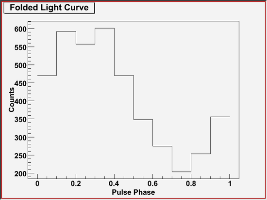
You can use gtptest to run several periodicity tests to check ephemeris information in the database is good for your dataset. It reads pulse phases that have just been assigned by gtpphase, performs statistical tests for periodicity on them, and displays the test results.
When successful, gtptest produces a test output and a graphical plot of a folded light curve on your screen. In this particular example, the following outputs will be displayed, showing a strong pulsation in the data.
Case 2: Refining Ephemerides in the Pulsar Ephemerides Database
Even if the entire database is not covered by the pulsar ephemerides database, you can still use it for your analysis by refining pulsar ephemerides in the database for your particular dataset. The first step of your analysis in this case is to find an ephemeris entry for your pulsar in the database.
You can run gtephem to check if your pulsar is listed in the pulsar ephemerides database. In the following example, gtephem searches for a pulsar by name and by observation time, computes estimated ephemeris of your pulsar at the observation time, and displays the result of computation. If it cannot find any ephemeris for your pulsar, it will produce a message stating it could not find any. In that case, you may need to try Case 3 or Case 4 described below.
With the successful result above, now you know at least one ephemeris is found in your database that can be used for your analysis. To find out how precise this ephemeris is at the time of your observation, you can run gtpsearch using the same pulsar ephemerides database.
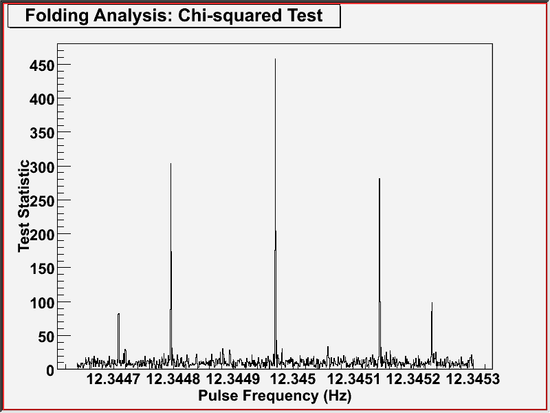
In the following example, gtpsearch reads the event file named fakepulsar_event.fits and performs periodicity tests called "chi-squared test" with 10 phase bins. Periodicity tests are performed at 100 trial pulse frequencies, which are automatically determined such that they are separated from each other by half a Fourier resolution, and that they center at the expected pulse frequency at the time origin of periodicity test, where the expected pulse frequency is determined by an pulsar ephemeris (or ephemerides) in the pulsar ephemerides database named bogus_pulsardb.fits for the pulsar named "PSR J9999+9999". As shown below, gtpsearch pops up a window showing a plot of test statistics as a function of frequency.

In this particular example, the maximum value of the chi-squared test statistic (a.k.a., S-value in the literature) appears at the exact center of the frequency range, because the ephemeris in the database is precise enough at the time of this observation. In general cases, though, the peak may show up in a different place in the plot.
Once you know the pulse frequency at the time of observation, you can use it as if it were taken from the literature in the following analysis, if you would like to. In that case, you may choose to assume all frequency derivatives to be negligible and set them to zero, or you may want to to determine frequency derivatives by yourself. For the former, continue on Case 3, and follow the description there with setting frequency derivatives to zeros. The latter case is beyond the scope of this tutorial and not described here.
Case 3: Using Pulsar Ephemeris in the Literature
You can run gtpsearch with specifying pulsar's spin parameters (pulse frequency or pulse period, and its time derivatives) by numbers, that are taken from the literature, for example.
In the following example, gtpsearch does the same thing as above, using 12.345, -2.345e-10, and 3.45e-20 for the pulse frequency and its first and second derivatives at the ephemeris epoch of 54870.0 MJD (TDB), respectively.
You can also run gtpphase with the same pulsar's spin parameters as above.
In the following example, gtpphase does the same thing as above, using 12.345, -2.345e-10, and 3.45e-20, for the pulse frequency, its first and second time derivatives at the ephemeris epoch of 54870.0 MJD (TDB), respectively.
Case 4: Determining Pulsar Ephemeris Yourself
If your pulsar is not listed in the database nor in the literature, you might want to determine ephemeris on your own by analyzing your data. One way to do it is to run gtpspec. In the following example, gtpspec reads the event file named fakepulsar_event.fits and performs Discrete Fast Fourier Transform (DFFT) with 10 ms time bins. The entire data set is broken up into data segments of 1,000,000 time bins (i.e., 100 ks in length), for each of which A DFFT will be performed and its Fourier power will be computed. Then, the Fourier powers of all the segments are summed up. The pulsar name "PSR J9999+9999" is used to look up for a binary orbital parameter in the pulsar ephemerides database named bogus_pulsardb.fits.
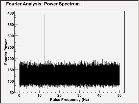
Frequency derivatives may be determined by running this tool multiple times with different combinations of frequency derivatives (given to the tool as ratios over frequency). Use caution when interpreting chance probability, because the tool can only compute it for the number of degrees for each run, not a set of runs with various frequency derivatives. You have to compute a correct chance probability for such analysis, based on the information displayed on the screen such as the number of independent trials for each run. The details on a full pulsation search are beyond the scope of this tutorial and not described here.
Once you determine the pulse frequency at the time of observation, you can use it in Case 3 as if it were taken from the literature in the following analysis.
4. Use Pulse Phases in Your Analysis
Sample File. To try the examples in this section, you can download the following fake data file:
- fakepulsar_event_phase.fits (408 kB)
Also see: Goddard Space Flight Center's:
|
If you have not already done so, download the FTOOL:
Note: You may also want to download: fplot, fv, and fdump.
Now you have a pulse phase number for each photon in your data. With those phase numbers, you can accumulate their distribution, or sub-select photons within a specific range of pulse phase.
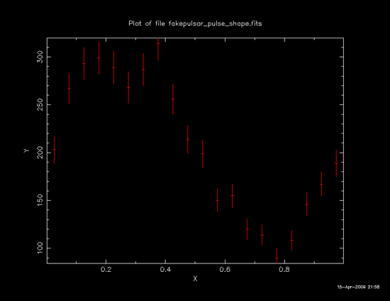
In the following example, fhisto (FTOOLS) creates a folded light curve, or a pulse shape, which is a distribution of values in PULSE_PHASE column of the event file named fakepulsar_event_phase.fits, assuming that the file has already been processed by gtpphase as described in Section 3, above: Calculate Pulse Phase for Each Photon. The distribution will be stored into a histogram with the bin size of 0.05 in phase for phase values ranging from 0.0 to 1.0, and written into an output FITS file named fakepulsar_pulse_shape.fits under the column names of X, Y, and Error.
Now you can display the pulse shape with your favorite plotting tool, such as fplot (FTOOLS, an example shown below) and fv (FTOOLS). You can also print the contents of the histogram in ASCII format by using fdump (FTOOLS).
| Owned by: Masaharu Hirayama |
| Last updated by: Masaharu Hirayama 04/17/2009 |