In this example, the LAT data is examined for a gamma-ray burst, based on the time and position derived from a GBM trigger.

SciTools Reference Pages: If you want the SciTools Reference pages to open in a popup window, click on: Open Popup Reference Window.

Assumptions

It is assumed that:

• You are running on SLAC Central Linux, and you are in your work directory.
  See Example: Setup (when running Science Tools on SLAC Central Linux).

• The GBM reported a burst via a GCN circular with the following information:
  • Name = GRB 080916C
  • RA = 121.8
  • Dec = -61.3
  • Tstart = 243216766 s (Mission Elapsed Time)
  • T90 = 66 s

Steps

1. Extract the Data

2. Data Selections

3. Bin the Data

4. Look at the Data

Generally, you should use the time and spatial information from some source (here, a GCN notice) then, from the SLAC Data Portal, use the Astro Server to make the appropiate extraction cuts. (See Data Access Help: Astro Server.)

For this exercise, use the following parameters and extract the data for an ROI of 40 degrees from 500s before to 1500 seconds after the trigger time:

• Search Center (RA,Dec) = (121.8,-61.3)
• Radius = 20 degrees
• Start Time (MET) = 243216266 seconds (2008-09-16T00:04:26)
• Stop Time (MET) = 243218266 seconds (2008-09-16T00:37:46)
• Minimum Energy = 20 MeV
• Maximum Energy = 300000 MeV

OR

You can download them here:

• exploreLATdata-ft2-30s.fits
• exploreLATdata-ft1.fits

To map the region of the burst, you should select a large region from within a short time range bracketing the burst. However, for the lightcurve, you should select a small region around the burst from within a long time range. Therefore, you will need to make two different data selections using, in both cases, the loosest event class cut in order to include all classes of events.

1. Use gtselect to extract the region for the spatial mapping:

Notes:

• The input photon file is exploreLATdata-ft1.fits, and the output file is GRB081916C_map_events.fits.

• We selected a circular region with radius 35 degree around the burst location (the ROI here has to fall within that selected in the data server) from a 300s time period around the trigger.

• We made an additional energy cut, selecting only photons between 100 MeV and 300 GeV to remove the low-energy, high-background events from the map.

2. Run gtselect again, this time with a smaller region but a longer time range. (Observe that gtselect saves the values from the previous run and uses them as defaults for the next run.)

prompt>  gtselect evclsmin=1 evclsmax=4
Input FT1 file[exploreLATdata-ft1.fits] 
Output FT1 file[GRB090119205_map_ph.fits] GRB081916C_lc_events.fits
RA for new search center (degrees) (0:360) [121.8] 
Dec for new search center (degrees) (-90:90) [-61.3]
radius of new search region (degrees) (0:180) [35] 10
start time (MET in s) (0:) [243216666] 
end time (MET in s) (0:) [243216966] 
lower energy limit (MeV) (0:) [100] 20
upper energy limit (MeV) (0:) [300000]  
maximum zenith angle value (degrees) (0:180) [180]
Done.
prompt>

Notes:

• A new output file, with the extension lc_events.fits has been produced.

• The search radius was reduced to 10 degrees.

• The start to stop time range has been expanded.

• The energy range has been expanded.

Use gtbin to bin the photon data into a map and a lightcurve.

1. Create the counts map:

prompt> gtbin
This is gtbin version ScienceTools-09-20-00
Type of output file (CCUBE|CMAP|LC|PHA1|PHA2) [] CMAP
Event data file name[] GRB081916C_map_events.fits
Output file name[] GRB081916C_counts_map.fits
Spacecraft data file name[NONE] 
Size of the X axis in pixels[] 50
Size of the Y axis in pixels[] 50
Image scale (in degrees/pixel)[] 0.5
Coordinate system (CEL - celestial, GAL -galactic) (CEL|GAL) [] CEL
First coordinate of image center in degrees (RA or galactic l)[] 121.8
Second coordinate of image center in degrees (DEC or galactic b)[] -61.3
Rotation angle of image axis, in degrees[0.] 
Projection method e.g. AIT|ARC|CAR|GLS|MER|NCP|SIN|STG|TAN:[] AIT
prompt>   

Note: Although in gtselect we selected a circular region with a 35 degree radius, we will form a counts map with 50 pixels on a side, and 0.5^o square pixels.

2. Create the light curve:

prompt> gtbin
This is gtbin version ScienceTools-09-20-00
Type of output file (CCUBE|CMAP|LC|PHA1|PHA2) [CMAP] LC
Event data file name[] GRB081916C_lc_events.fits
Output file name[] GRB081916C_light_curve.fits
Spacecraft data file name[NONE] 
Algorithm for defining time bins (FILE|LIN|SNR) [] LIN
Start value for first time bin in MET[] 243216266
Stop value for last time bin in MET[] 243218266
Width of linearly uniform time bins in MET[] 10
prompt>   

Notes:

• gtselect was used to create GRB081916C_lc_events.fits, a photon list from a small region, but within a long time range.

• gtbin will bin these photons and output the result into GRB081916C_light_curve.fits.

There are a number of options for choosing the time bins. Here we have chosen linear bins with equal time widths of 10 seconds.

We now have two FITS files with binned data:

• GRB081916C_light_curve.fits
• GRB081916C_counts_map.fits

To look at the count map:

1. At the command line, enter: fv GRB081916C_counts_map.fits

A new GUI will open:

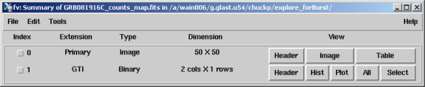
2. In the Summary Window for the FITS file, click on the Image button. 

Note: FITS files consist of a series of extensions with data. Since the counts map is an image, it is stored in the primary extension (for historical reasons only images can be stored in the primary extension). Clicking on the 'Image' button in the first row results in:

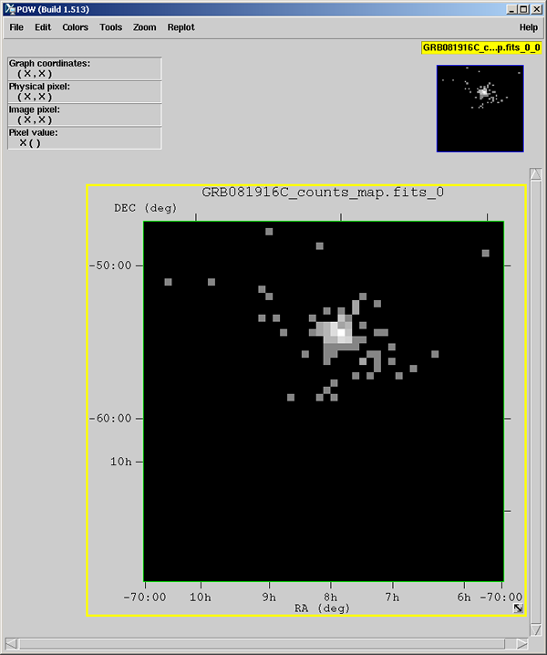
Observe that there are many pixels containing a few counts each near the burst location, and few pixels containing any counts away from the burst. Note also that the burst location is not centered in the counts map, which means that the preliminary location sent out in the GCN was not quite the right location; this is not uncommon for automated transient localizations.

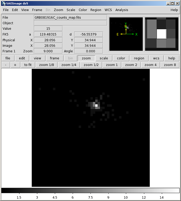
3. Use ds9 to look at the counts map; at the prompt enter:

   ds9 GRB081916C_counts_map.fits

   Tip: To change the ds9 display for the mouseover from sexagesimal (the default) to degrees, go to the WCS menu and select Degrees.

4. Mouse over the brightest pixel.

The RA and Dec (119.5, -56.5, respectively) of the likely burst location will be displayed in the FK5 boxes. Though not as accurate as fitting the data (see the Likelihood Tutorial), this is a quick method of localizing a burst.

To look at the lightcurve:

1. Enter (at the prompt): fv GRB081916C_light_curve.fits

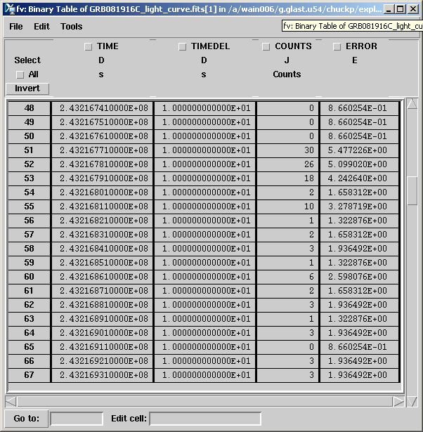
The lightcurve is in the RATE extension, which has 4 columns: TIME, TIMEDEL, COUNTS and ERROR.

2. To view the content of the RATE extension, click on: All

Note: The time bins were created to have a width of 10 s, and therefore TIMEDEL is always 10.

RATE Extension GUI:

3. To plot the COUNTS as a function of TIME. From the RATE Extension GUI's Tools drop-down menu, select: Plot

   The following GUI will be displayed (select TIME, then click on X; then select COUNTS and click on Y):

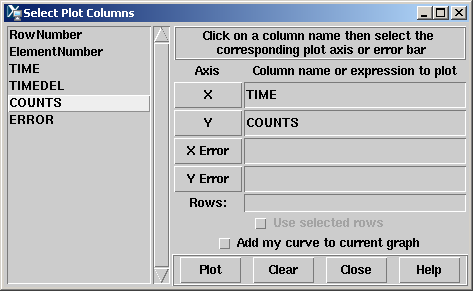
3. Click on the Plot button.

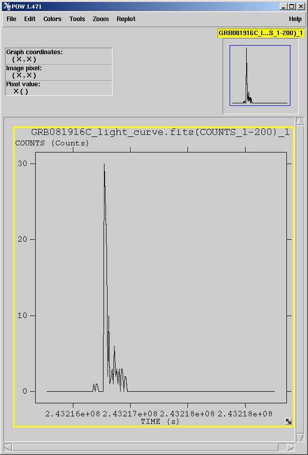
Note: Except for the burst, almost all bins have 0 counts, with only an occasional bin with one count. This demonstrates that there is essentially no background for LAT observations of gamma-ray bursts.