This document is intended to help SLAC physicists, operators and users, to write Matlab software for data analysis, control, and optimization, of the LCLS-II accelerator complex.
This documents is a WORKING DRAFT. This version incorporates code review.
Please see Addendum Items to be Added to the Document, for list of items planned but not yet included. A Python version is intended to follow, but as of 08-Nov-2023 has not yet been prepared.
This HTML file is in git repo /afs/slac/g/cd/swe/git/repos/sites/www.slac.stanford.edu/grp/ad/docs/model/matlab.git.
To update this document and republish to the web; git clone matlab.git
above, make changes, and simply git add, commit and push as you would. The git push will
immediately and automatically republish the head to
https://www.slac.stanford.edu/grp/ad/docs/model/matlab/. Full instructions
are in the Cheat sheet
for using git for web sites hosted by basic SLAC web server
There is a published set of Matlab Programming Standards which covers the basics of how one should write actual Matlab code (syntax, organization, commenting etc.). Please adhere to those standards when developing SLAC production Matlab code.
This document assumes Matlab HLA development is carried out on the production network (as has been common practice). In a future version of this document, application development on AFS and one's own machine will be described
To develop applications software for LCLS, you will need at least the following:
To login to the production network, with the prerequisites above in place, login to lcls-srv01.slac.stanford.edu using the physics user name. You must go via the mcclogin host. The following one line, executed from SLAC public AFS machine rhel6-64, would make a fast login to lcls-srv01 using tricks for encryption and compression that can make lclshome and apps run acceptably fast over X11 on most modern networks. You may also use fastx or NX to get to a SLAC public host. From there login to mcclogin, and then to lcls-srv01.
  [greg@rhel6-64e ~]$ ssh -A -t -Y -C -l<your-slac-username> mcclogin.slac.stanford.edu \
  ssh -A -t -Y -C -l physics lcls-srv01
At the prompt, declare who you are, as you agreed with Mike above. For me it's "greg".
This section describes starting Matlab - the primary data analysis and physics application development tool we use in the online LCLS control system.
On production, if you want the full graphical development environment of the default matlab version (presently Matlab 2020a), simply type matlab at the prompt. If you want to run applications only, or just do some basic scripting, add the nodesktop option. nosplash makes Matlab start a bit faster. There is also a script run_matlab.bash, which is used to launch matlab applications from lclshome. It takes a matlab version argument (-m). Use run_matlab.bash if you want to emulate the environment in which a GUI would be launched, in the version of Matlab under which it is launched.
[physics@lcls-srv01] $ matlab   Full Matlab GUI environment of the default Matlab version
[physics@lcls-srv01] $ matlab -nodesktop -nosplash   In-terminal matlab of default Matlab version
[physics@lcls-srv01] $ run_matlab.bash -m 2012a   In-terminal Matlab as used to launch ver 2012a apps
Note though that, at the time of writing, our Matlab GUIs have all been developed with Matlab Guide (the old GUI building system of Matlab) and so far we have little experience of it's replacement, App Designer. There is a conversion tool. See Mathworks pages to help one Create apps with graphical user interfaces in MATLAB.
On production LCLS hosts (lcls-srv01 etc), our matlab files are primarily to be found
in directories under /usr/local/lcls/tools/matlab (environment variable
$MAT):
/usr/local/lcls/tools/matlab/toolbox   Physics and apps oriented
/usr/local/lcls/tools/matlab/src       Support, utilities, controls oriented
The full list of directories Matlab looks in to find scripts and functions, can be found by typing path at the Matlab prompt.
Note: Our Matlab startup.m file is set up to automatically put all subdirectories it finds under /usr/local/lcls/tools/matlab/toolbox also on the matlab path. Therefore, it makes sense to put new projects in their own subdirectory.
Both toolbox and src are kept in our CVS based source code management system, see below.
CVS (Code Versioning System) bib:cvs is a way of keeping track of changes to code. It's especially helpful in a software development collaboration. You can use CVS to keep track of changes to your scripts, enable collaborative editing, and compare to previous versions, etc.
Our CVS at SLAC keeps track of all the software that runs the LCLS accelerator complex, is in a single so called, "repository" called "LCLS". The repository is subdivided into "modules" - essentially directories of files.
Our Matlab files are in the matlab CVS repository
In outline, the procedure is you work with copies of these files in your working
directory. You first "checkout" matlab/src or matlab/toolbox
from the repository to your working directory. You make changes to the files, or add
files. When you're ready to release your version, so that the control system and your
colleagues can use it, you "commit" it to the repository, and then "update" the shared
directory that contains all the files of the matching module
(/usr/local/lcls/tools/matlab/toolbox or
/usr/local/lcls/tools/matlab/src). At that point, everyone else, and LCLS,
will be using the files you contributed. See below for the step-by-step commands.
CVS references: See Cheatsheet section on CVS commands.
This section describes typical actions you might take to develop a Matlab HLA for the LCLS accelerators. Note, this is a little different to the old Matlab development workflow. This workflow specifically enables you to have more than one project in development at the same time, all under your home directory (like ~physics/greg/) but not interfering with each other.
The following pattern is appropriate for minor modifications to a single file, or large multi-week projects.
Begin by creating a directory to do your development, and another
beneath that specifically for your cvs files.
Then checkout matlab files you want to work on. You can choose to
checkout one or more individual files- giving the whole filename, or
checkout all of matlab/toolbox/.
~/greg/Development]$ mkdir myproject
~/greg/Development]$ cd myproject              # Keep associated files/docs here
~/greg/Development/myproject]$ mkdir lclscvs
~/greg/Development/myproject]$ cd lclscvs/     # CVS files here

~/greg/Development/myproject/lclscvs]$ cvs co matlab/toolbox/meme/src/meme_names.m
greg@mcclogin's password:
U matlab/toolbox/meme/src/meme_names.m
or checkout everything in toolbox
~/greg/Development/myproject/lclscvs]$ cvs co matlab/toolbox
…
Now to tell Matlab where your development matlab files can be found. You can either
use the "Set Path" preference inside matlab every time you open matlab, or copy startup.m
to your project directory and edit it. In this latter way, you can keep a number of
matlab project folders, and just start matlab from the appropriate directory - the one
containing startup.m - for that project.
~/greg/Development/myproject/lclscvs]$ cd ..
~/greg/Development/myproject]$ cp $MAT/toolbox/startup.m .    # don't forget the "."
~/greg/Development/myproject]$ chmod +w startup.m             # change permissions so can modify it
Using the startup.m way, edit startup.m to assign the special variable USERPATHROOT towards the top of the file (you will find examples in startup.m) and set it to the root directory of your matlab files. The startup.m file has code in it to add all the directories below the directory you name, to your path. You can edit it with emacs or Matlab itself - but if using matlab, be sure to restart matlab so it executes your local startup.m. Find the part of startup.m where you would add your USERPATHROOT and add it. There must be 0 or 1 USERPATHROOT in the file, so leave others and examples commented out:
% Wire-scan and emittance
%  USERPATHROOT='/home/physics/greg/Development/emit/lclscvs/matlab';
% Where I develop myproject matlab files. Ie where I checked out matlab/toolbox/ files to.
  USERPATHROOT='/home/physics/greg/Development/myproject/lclscvs/matlab';
Now, whenever you start matlab from the myproject directory (which contains your edited startup.m) your project files will be at the top of matlab's path.
~/greg/Development/myproject]$ matlab &
There is a short administrative procedure for reviewing and releasing SLAC accelerator online software, which includes Matlab. The procedure is described in Appendix B: Software Release Procedure. That procedure ensures that new software is reviewed, does not disrupt beam operations, maintains software quality, and includes a provision to test beam physics related software with beam. Follow the procedure as described in the Appendix. The section below is just about the mechanics of the matlab file deployment into production. You would do the two steps below in the last item of the procedure described in the Appendix.
When you have completed a project, follow the following steps to release it. You can
then delete the project directory, or keep it around (together with notes in your
myproject directory). The following is an example of releasing modifications I made to
matlab/toolbox/meme/src/meme_names.m .
Before release check that your change does affect any other matlab. If you have chnaged input or output parameters, or error handling in any way, verify all m-file callers of your changed m-files are compatible with your change or have been modified to accept your change.
~/greg/Development/myproject/lclscvs/matlab/toolbox/meme/src]$ ls
total 4
-rw-rw-r-- 1 physics lcls 1581 Jan 31 18:37 meme_names.m
drwxrwxr-x 2 physics lcls    6 Jan 31 14:50 CVS
~/greg/Development/myproject/lclscvs/matlab/toolbox/meme/src]$ cvs commit -m "removed name arg" meme_names.m
greg@mcclogin's password:
Checking in meme_names.m;
/afs/slac/g/lcls/cvs/matlab/toolbox/meme/src/meme_names.m,v  <--  meme_names.m
new revision: 1.3; previous revision: 1.2
done
~/greg/Development/myproject/lclscvs/matlab/toolbox/meme/src]$ cvs2prod
greg@mcclogin's password:
U meme/src/meme_names.m
Completed, the new meme_names.m is now in production and all production apps will use the new version.
This section describes how your matlab can interface to the control system.
Most of the control system software used for LCLS and other SLAC accelerators, is based on EPICS (Experimental Physics and Industrial Control System) bib:epics.
EPICS uses two means of communication (or "network protocols") to talk to the devices of the accelerator; the legacy "Channel Access" protocol, and the new "pvAccess" protocol.
As a user, to get device's data or to make a device go to a value, you perform get and set operations on a so-called "Process Variable", or "PV" for short. When you refer to a PV, you refer simply to its name. A PV name is simply the ASCII string that identifies the process variable quantity. Think of PVs as an entity-attribute-value system. At SLAC, when the value refers to a control system device setpoint or readback, the entity is the name of the device (eg QUAD:IN20:941, the attribute is some control or readback quantity of the device, such as magnet's BDES, and the value is the control or readback value. The SLAC PV naming convention makes this really clear for devices and their attributes.
| Entity / Device Name | Attribute | PV name |
|---|---|---|
| QUAD:IN20:941 | BDES | QUAD:IN20:941:BDES |
EPICS version 4 (now called version 7!) introduced the pvAccess protocol. pvAccess can do everything that Channel Access can do, and it adds 2 large feature sets: it can handle complex structured data (for instance 1 PV can carry all the data and metadata of an areaDetector NDArray), and it can handle PVs whose values are subject to arguments supplied at runtime - like a function call.
Since EPICS version V7 PVs can carry complex data, often not oriented towards a single device, some EPICS V7 PV names are not <device-name>:<attribute-name>. For instance, some PVs refer to the whole of LCLS, so they're prefixed "LCLS".
At the time of writing, SLAC only uses the new pvAccess protocol for complex process variables - those whose values are tables, or matrices, or self-describing images, rather than simple scalar or array values.
| Example PV name | Content | Protocol | Matlab APIs | Python APIs |
|---|---|---|---|---|
| QUAD:IN20:941:BDES | A float giving the field setpoint of quadrupole QUAD:IN20:941 | CA | labCA or eget.m | pyepics |
| BMAD:SYS0:1:CU_HXR:LIVE:TWISS | A table of the live Curant-Snyder parameters of all devices | PVA | eget.m | p4p |
The labCA toolbox wraps the essential ChannelAccess routines and makes them accessible from the MATLAB programs.
For details of lca see the reference manual, "labCA -- An EPICS Channel Access Interface for scilab and matlab."
All labCA calls take a PV name argument identifying the EPICS process variable, or array of process variables, the user wants to access. EPICS PVs are plain ASCII strings that follow the < device-name > : < attribute-name > pattern described above. Note that labCA cannot be used to access process variables that are only available over EPICS 7 pvAccess.
LabCA is capable of handling multiple PVs in a single call; they are simply passed as a cell-array of strings, e.g.:
pvs = { 'QUAD:IN20:941:BDES'; 'QUAD:IN20:941:BACT'; 'QUAD:IN20:941:EACT' }
Unless all the PVs in an lca call are of EPICS native string type (or more formally "char") or conversion to char is enforced explicitly, labCA always converts data to double. Legal values for type are byte, short, long, float, double, native, or char (for strings).
ChannelAccess timestamps provide the number of nanoseconds since 00:00:00 UTC, January 1, 1970. LabCA translates the timestamp into a complex number with the seconds in the real and nanoseconds in the imaginary parts.
To convert timestamps into MATLAB format use lca2matlabTime (see example for lcaGet below.There are 2 kinds of things that can go wrong in an EPICS PV interaction like lcaGet and lcaPut. The first are related to the computation itself, like a typo in the pv name, or the EPICS record in the IOC associated with that PV isn't available on the network. Such problems result in matlab exceptions. The second are oriented toward the validity of the data or control action or IOC connection to its device hardare. This second kind are handled through the EPICS alarm "status" and "severity." EPICS severity value of "INVALID" indicates EPICS detected an internal error. Schematically;
yourlcamatlab <--ca--> IOC <--fieldbus--> hardware
These two error types and their handling are further described below.
If lca can't contact a PV, or otherwise can't complete an I/O operation, it throws an exception. If the exception is not "caught", the execution is aborted (look for details in the MATLAB manual). That is, if there is no catch statement anywhere in the stack of functions that the matlab process has executed so far to get to your lcaGet, then your matlab program will crash. So, you should always program with try-catch blocks around any lca code that can fail.
The generic code pattern for the handling of lca operations like lcaGet and lcaPut is given at https://www.slac.stanford.edu/grp/ssrl/spear/epics/extensions/labca/manual/node4.html#errorhandling. That page includes also a table for proper interpretation of the status codes from lcaLastError. The Matlab specific equivalent is below:
STDERR=2; % The file-id corresponding to the unix standard error

try
    lcaPut('invalidlynamedpv',1);    %! A pv invalid by virtue of something like wrong name, or offline IOC
catch ex
    errcodes = lcaLastError(); %! Get the error code (or if >1 PV) codes, see lca error codes table
    fprintf(STDERR, 'errorcodes %i\n', errcodes ); % Print the error code
    fprintf(STDERR, '%s\n', getReport(ex,'extended'));  % Print extended error message
end
An example execution of the above code is below. Note the getReport()
prints 6 lines (including blank lines):
errorcode 6
Error using lcaGet
multi_ezca_get_nelem -  ezcaGetNelem(): could not find process variable :invalidlynamedpv

Error in putsmarttest (line3)
   val=lcaGet('invalidlynamedpv');
This same basic pattern is valid for lca operations generally, like lcaGet and lcaPut, lcaGetStatus. etc.
A more complete exception handling pattern is given below.
The second kind of PV errors are related to the IOC, its communications to harward and
its record processing. These are problems like the PV is out its control limits. The
basic call to get a PVs status and severity is
lcaGetStatus . Basic references are the EPICS
Record Reference Manual,
Alarm Specification.
The possible values of alarm SEVR and STAT are defined in: https://github.com/epicsdeb/epics-base/blob/master/src/libCom/misc/alarm.h
NOTE: Our lcaInit.m sets the so called "severity rejection level" to None, by setting value 14! That is to say, calls to lcaGet will therefore NOT return NaN in cases that the VALue of the PV is bad in any way, even disconnected hardware! For instance, by default, your code is NOT warned if the value is below the LOLO status value, which is a MAJOR alarm condition. cf lcaInit.m
The consequences are described below by example of a PV whose value is, at the time of writing, out of tolerance.
For instance at the time of writing, the value of PV KLYS:DMPH:1:MICROPERVEANCE is
too low. It's 0 and it should be more than 0.95 (see KLYS:DMPH:1:MICROPERVEANCE.LOLO):

>> uperv = lcaGet('KLYS:DMPH:1:MICROPERVEANCE')

uperv =
      0

That value of 0 in fact puts the PV in LOLO status, which in the case
of this PV is a MAJOR severity alarm (see below):

>> [sv,st,~]=lcaGetStatus('KLYS:DMPH:1:MICROPERVEANCE')

sv =
      2

st =
      5

You can get access to the SEVeRity and STATus also from the PV's SEVR and STAT fields:

>> lcaGet('KLYS:DMPH:1:MICROPERVEANCE.SEVR')

ans =

    'MAJOR'   % epicsAlarmSeverity = MAJOR_ALARM = 2

>> lcaGet('KLYS:DMPH:1:MICROPERVEANCE.STAT')

ans =
    'LOLO'   % epicsAlarmCondition = LOLO_ALARM = 5
We can set LCA's "Severity rejection level" so that the returned value will be NaN rather than the questionable value of the PV's VAL field when the PV's severity is above a given threshold. For instance, with the KLYS:DMPH:1:MICROPERVEANCE PV still in MAJOR severity due to its low value of 0, as above:
>> lcaSetSeverityWarnLevel(12)
Setting severity REJECTION level to 2

>> v=lcaGet('KLYS:DMPH:1:MICROPERVEANCE')

v =

   NaN

Then we can set it back to 14 when we have completed the lca operation that needed
to be warned of a non-0 severity

>> lcaSetSeverityWarnLevel(14)
Setting severity REJECTION level to 4
>> v=lcaGet('KLYS:DMPH:1:MICROPERVEANCE')

v =

     0
Since labCA is used for accessing data via network, your function calls can timeout (see 2.4).
lcaGet is the basic function use to get the values of EPICS process
variables over Channel Access. The value of one or a number of Process Variables can be
acquired with one call. See lca reference manual, lcaGet.
[value, timestamp] = lcaGet(pvs, nmax, type)
'byte', 'short', 'long', 'float', 'double', 'native',
'char'
.
>> % Get the desired and actual B fields of a corrector
>> [values, timestamps] = lcaGet({'XCOR:LI22:402:BDES';'XCOR:LI22:402:BACT'});
>> values
values =

   0.0012
   0.0012

>> datestr(lca2matlabTime(timestamps))

ans=

   10-Jan-2018 10:17:55
   10-Jan-2018 11:38:23
See also the Lca User Guide for examples of using lcaGet.
lcaPut and lcaPutWait functions write values to PVs. The PVs may be scalars or arrays of different dimensions. It is possible to write the same value to a collection of PVs.
lcaPut will wait until the request is processed on the server, whereas lcaPutNoWait returns immediately.
lcaPut(pvs, value, type)
lcaPutNoWait(pvs, value, type)
>> lcaPut('XCOR:LI22:402:BDES', 0.00125)
>> lcaGet('XCOR:LI22:402:BDES')
ans =
0.00125
See also the Lca User Guide for examples of using lcaPut, and lcaPutNoWait.
Get the names of the
The MAD "decks" for LCLS, LCLS-II and FACET beampaths, are available on the web at https://www.slac.stanford.edu/grp/ad/model/. Specifically:
| Decks | URL |
|---|---|
| Operational LCLS accelerator | https://www.slac.stanford.edu/grp/ad/model/lcls.html |
| Planned LCLS High Energy (HE) accelerator | https://www.slac.stanford.edu/grp/ad/model/lcls2he.html |
Note the Beampaths section of the MAD deck web sites above. They list the distinct electron beam traversals possible in "LCLS".
| Beampath | The top level of organization of LCLS is "beampath." A beampath is a complete electron traversal from one of the cathodes to a dump. The MAD deck defines 8 beampaths now, eg SC_SXR, SC_HXR, CU_HXR etc. |
| Line | Within a beampath is a hierarchy of lines (lines may contain lines). For instance the CU_HXR beampath (as implemented for LCLS) starts with GUN, then L0, DL1_1, DL1_2, L1 and so on. |
| Device names | Every MAD deck element that has an assigned device name. The modelled devices of beampath CU_HXR are listed, by their line, in LCLS2cuH_lines.dat |
We have two primary Matlab functions for getting device names; model_nameRegion.m, which takes it names from model_nameList.m, and is integrated into the matlab model, bib:HLA_swlist, and meme_names.m which directly integrated into the main MAD decks, and hence the Directory Service, Oracle and BMAD. Other things being equal, the two systems should give largely teh same names. There are some differences in the names associated with cavities and bends.
model_nameRegion is the basic mechanism to get names from the matlab model system. It understands device types, beampaths, and area names. E.g. to find the (two) BPMs in GUNB (the first area of the SC beampaths:
>> model_nameRegion('BPMS','GUNB')

ans =

  2x1 cell array

    {'BPMS:GUNB:314'}
    {'BPMS:GUNB:925'}
model_nameConvert is the old matlab function for getting PV names and converting element names to device names. It also knows areas, see LTUH example below:
>> model_nameConvert('BPMS:LTUH:120','MAD')

ans =

BPMVM2

>> names=model_nameConvert({'XCOR','YCOR'},'EPICS','LTUH')    % correctors device names in LTUH

names =

  37x1 cell array

    {'XCOR:LTUH:115'}
    {'XCOR:LTUH:178'}
    {'XCOR:LTUH:144'}
     ...
The meme_names.m Matlab function is the new function to get names of PVs,
devices, and elements. meme_names knows the LCLS Cu and SC accelerator
beampaths and their Areas, as defined in the Beamline
Boundaries PRD Table 3. Beampaths and Areas are known to the directory service
collectively as lname (for line name). Directory Service also knows the MAD element type
(etype) of all lattice related devices, and hence PVs. The MAD element types are SLAC's
extensions of the MAD8 types (see the MAD 8 Users Guide bib:MAD8UG Table A.1). The most common at SLAC are: MONI (bpm), HKIC (xcor), VKIC (ycor),
QUAD (quad), LCAV (cavity). The default is to return all
matching PV names, but you can specify what to return with the 'show'
argument. To see formally what the types of each element in MAD, see the relevant lines
files in the beampaths table of
the LCLS lattice web page.
Using 'lname' argument to meme_names to get all the modelled devices in a Beampath. The following gets all the modelled devices in SC_SXR, in z order:
>> meme_names('lname','SC_SXR','show','dname','sort','z')
To show the device names of MONItors (ie BPMs in MAD speak) in the SC GUN (in fact there are only 2):
>> meme_names('etype','MONI','lname','GUNB','show','dname')    % BPMS in the GUN, return device names

ans =

  2x1 cell array

    {'BPMS:GUNB:314'}
    {'BPMS:GUNB:925'}
The Areas are specifically defined to be conjoined and non-overlapping. In this way you can build up a device list of a section of the accelerator through concatenated areas. So for instance, these are the BPMS in the areas GUNB through L0B and HTR.
>> [meme_names('etype','MONI','lname','GUNB','show','dname');meme_names('etype','MONI','lname','L0B','show','dname'); ...
meme_names('etype','MONI','lname','HTR','show','dname')]

ans =

  13x1 cell array

    {'BPMS:GUNB:314'}
    {'BPMS:GUNB:925'}
    {'BPMS:L0B:0183'}
    {'BPMS:HTR:120' }
    {'BPMS:HTR:320' }
    {'BPMS:HTR:365' }
    {'BPMS:HTR:460' }
    {'BPMS:HTR:540' }
    {'BPMS:HTR:760' }
    {'BPMS:HTR:830' }
    {'BPMS:HTR:860' }
    {'BPMS:HTR:960' }
    {'BPMS:HTR:980' }
Additionally we may ask not for the device names, but the PV names. Every device has many PV names, so meme_names accepts a wildcard pattern. The basic wildcard is '%'. So, for the devices' PV names which end in :X, rather than the device names themselves with 'name','%:X'. There are not many at the time of writing for SC, a year prior to commissioning, because although we have the device names in MAD and Oracle, not many EPICS PVs are yet known ot the control system:
>> [meme_names('etype','MONI','lname','GUNB','name','%:X');meme_names('etype','MONI','lname','L0B','name','%:X'); ...
meme_names('etype','MONI','lname','HTR','name','%:X')]

ans =

  4x1 cell array

    {'BPMS:GUNB:314:FW:X'}
    {'BPMS:GUNB:314:X'   }
    {'BPMS:GUNB:925:FW:X'}
    {'BPMS:GUNB:925:X'   }
To get all the X related PV names of BPMS:GUNB:314
>> meme_names('name','BPMS:GUNB:314:X%')
This example returns all the PVs of a given X corrector using a simple wildcard '%':
>> meme_names('name','XCOR:LI21:101:%')
PV names matching regex patterns. This gives PHAS PVs of all KLYS:
>> meme_names('regex','KLYS:[A-Z]{2,3}[0-9]{1,2}:[0-9]{1,4}:PHAS')
BPM device names in the Area named LTUS:
>> meme_names('etype','MONI','lname','LTUS','show','dname')
All BPM PV names in LTU. The default is to show the PV name. This will be a very long list:
>> meme_names('etype','MONI','lname','LTUH')
The BPM PV names in the first CLTH area, that also match the basic pattern '%:XTH'. The XTH PVs of BPMS are those that update at 10 Hz. So these are the X offsets of the BPMS in CLTH_1 read at 10 Hz:
>> meme_names('etype','MONI','lname','CLTH_1','name','%:XTH')
Get all the LCLS BSA rootnames, sorted by Z. Then get the PV names corresponding to one of those root names.
>> meme_names('sort','z','tag','LCLS.BSA.rootnames','lname','CU_HXR')  % Get sorted rootnames of BSA
devices in CU_HXR line
>> meme_names('name','VPIO:IN20:W770:FASTP%')         % Get PV names of one rootname
meme_names.m uses the new EPICS Directory Service for its data, which in turn gets data from the lines files created as part of the MAD lattice release process, and the IOCs themselves. You can also use command line EPICS 7 tools (eget) and Python to access the same data. See Greg's cheatsheet file memeExamples.txt bib:memeex gives many more examples (see section 3).
There are two of basic interfaces to 1st order optics presently in our Matlab;
>> modelSource = 'MATLAB';
model_rMatGet.m is the workhorse R-matrix acquisition engine of HLA software. It uses the Matlab implementation of the MAD device descriptions (by default, or if modelSource explicitly set to MATLAB as above).
>> help model_rMatGet
    [RMAT, ZPOS, LEFF, TWISS, ENERGY] = model_rMatGet(NAMELIST, NAMETO, OPTS, PARAM)
  gets transport matrix RMAT, z position ZPOS, effective length LEFF, Twiss
  params TWISS [energy phi_x beta_x alpha_x eta_x eta'_x phi_y ... eta'_y]'
  and energy ENERGY for devices in string or cellstr array NAMELIST.
  ...
NAMELIST should give a device name, as a matlab char string name, or an array of device names as a cell array of strings. If NAMETO (below) is not given, the R-matrix from the cathode to NAMELIST device(s) is returned. If NAMETO is given, the R-matrices from NAMELIST to NAMETO are returned.
OPTS allows you to specify whether you want the Twiss and R-mats computed from the nominal settings of the devices (TYPE=DESIGN), or the Twiss and R-mats computed from the existing PV values (TYPE=EXTANT). The extant, from PVs' values, is the default.
OPTS also is the way to specify the beampath of interest (per the Beamline Boundaries PRD Table 3, Path column). CU_HXR is the default.
In summary:
| Argument | Meaning | Default |
|---|---|---|
| NAMELIST | Names of devices for which to get model. If no NAMETO, returned Rmats are from Cathode | Required |
| NAMETO | Names of devices for which to get model. If given, the Rmats from NAMELIST devices to NAMETO devices are returned | Optional |
| OPTS TYPE={DESIGN|EXTANT} | Model computed from nominal constant magnet and RF settings (DESIGN), or from real PVs (EXTANT) | EXTANT |
| OPTS BEAMPATH={SC_SXR| SC_SFTS| SC_SXTES| SC_HXR| SC_BSYD| SC_DIAG0| SC_DASEL| CU_HXR| CU_SFTH| CU_HXTES| CU_SXR| CU_ALINE| CU_GSPEC| CU_SPEC| F2_ELEC| F2_SCAV| F2_POSI} | Model computed from nominal constant magnet and RF settings (DESIGN), or from real PVs (EXTANT) | CU_HXR |
For instance, get the R-matrix of a given device (from the head of the machine), from the model's DESIGN RF and magnet Ks:
>> modelSource = 'MATLAB';
>> model_rMatGet('BPMS:GUNB:314',[],{'BEAMPATH=SC_HXR','TYPE=DESIGN'})

ans =

    1.0000    0.4896         0         0         0         0
         0    1.0000         0         0         0         0
         0         0    1.0000    0.4896         0         0
         0         0         0    1.0000         0         0
         0         0         0         0    1.0000    0.0804
         0         0         0         0         0    1.0000
The default is to compute the CU model, and from CURRENT PV values
>> model_rMatGet('BPMS:LI21:233')  % or model_rMatGet('BPMS11')

ans =

   -0.6720   -0.2513         0         0    5.0546    0.0513
    0.0226   -0.0314         0         0   -0.0321   -0.0002
         0         0    1.4268    3.5996         0         0
         0         0    0.4279    1.0985         0         0
   -0.0034    0.0090         0         0    0.5375    0.0068
   -0.0406   -0.0326         0         0  -20.5741   -0.2111
(Note: When the machine is not running, you can run epicsSimul_init prior to running model_rMatGet to get somewhat meaningful numbers (see Fakedata below).
Get the DESIGN model R-Mats for the same device:
>> model_rMatGet('BPMS:LI21:233',[], 'TYPE=DESIGN')

ans =

   -0.6733   -0.2519         0         0    5.0560    0.0513
    0.0228   -0.0313         0         0   -0.0321   -0.0002
         0         0    1.4261    3.5967         0         0
         0         0    0.4276    1.0977         0         0
   -0.0035    0.0089         0         0    0.5374    0.0068
   -0.0405   -0.0325         0         0  -20.5800   -0.2111
You can give a cell array of strings to get a system of matrices:
>> model_rMatGet({'BPMS:LI21:233', 'BPMS:LI24:801', 'BPMS:LTUH:250'})

ans(:,:,1) =

   -0.0829    0.8827         0         0    4.9944    0.0523
   -0.0247   -0.0267         0         0   -0.0000    0.0000
         0         0    0.4311   -0.0466         0         0
         0         0    0.2268    0.0312         0         0
    0.0057    0.0062         0         0    0.5751    0.0071
   -0.0000    0.0000         0         0  -21.6137   -0.2262


ans(:,:,2) =

   -0.0919    0.5876         0         0    3.3327    0.0560
    0.0037   -0.0387         0         0    0.0000    0.0000
         0         0    0.0923    0.0913         0         0
         0         0   -0.0026    0.0126         0         0
   -0.0013    0.0140         0         0    0.0377    0.0008
    0.0000    0.0000         0         0   -9.2052   -0.1545


ans(:,:,3) =

   -0.0334    0.1669   -0.0000   -0.0000   -0.3627   -0.0061
   -0.0032    0.0027   -0.0000   -0.0000   -0.0000   -0.0000
   -0.0000   -0.0000   -0.0627   -0.0515    0.0000    0.0000
   -0.0000   -0.0000    0.0066   -0.0016    0.0000    0.0000
   -0.0004    0.0003   -0.0000   -0.0000   -0.0759   -0.0011
    0.0000    0.0000         0         0   -2.9019   -0.0487
The Rmat from A to B (by default from MATLAB extant model):
>> model_rMatGet('XCOR:LI21:135','BPMS:LI21:301')
model_twissGet.m is the equivalent method for getting Twiss data:
model_twissGet
  [TWISS, SIGMA, ENERGY, PHASE] = model_twissGet(NAME, ROPTS, OPTS) returns
  Twiss parameters TWISS, SIGMA matrix elements, ENERGY and PHASE for beam line
  elements in NAME.  Options for model_rMatGet can be specified in ROPTS,
  and further options in OPTS.
The 3×2 TWISS matrix returned is [emitnx emitny; betax betay; alphax
alphay]. Some examples of Twiss model:
>> % Get twiss computed from live PV values from Matlab internal MAD based model, of (default)
CU_HXR beampath
>> model_twissGet('BPMS:LI21:233')

ans =

    0.0000    0.0000
   73.4498  857.5393
   -1.6339 -283.7548

>> % Get design twiss, signal matrix, Energy and phase advance, from Matlab internal MAD based
model, using default element control system values (ie design model) for explicitly CU_HXR beampath
>> [t,sig,E,psi]=model_twissGet('BPMS:LTUH:730',{'BEAMPATH=CU_HXR','TYPE=DESIGN'})

>> % Get a system of Twiss parameters
>> model_twissGet({'BPMS:LI21:233', 'BPMS:LI24:801', 'BPMS:LTUH:250'});
In addition to the internal Matlab model, we have a continuously running EPICS 7 service, which computes and publishes R-mats and Twiss of all lattice devices as EPICS 7 NTTable PVs:
These model PVs are accessible from the bash command line (with for instance pvget or eget) or inside Matlab with eget.m.
| pvAccess PV name | Description |
|---|---|
| BMAD:SYS0:1:CU_HXR:LIVE:TWISS | The Courant Snyder parameters of all lattice elements of the CU_HXR beampath as computed from device PVs continuously, given as 9 column Matlab Table, of eg 'alpha x', 'beta x' etc. |
| BMAD:SYS0:1:CU_HXR:DESIGN:TWISS | Design Courant Snyder parameters of all lattice elements of the CU_HXR beampath, with the same columns as the extant equivalent above |
| BMAD:SYS0:1:CU_HXR:LIVE:RMAT | Coupled 6x6 transport matrices of all lattice elements of the CU_HXR beampath, given as 40 column Matlab Table, one row per 6x6 matrix plus 4 columns, eg 'device_name', 'r12', 'r66' etc) continuously computed from the control system PVs. Each matrix represents the translation from the nominal cathode to the device |
| BMAD:SYS0:1:CU_HXR:DESIGN:RMAT | The design coupled 6x6 transport matrices of all lattice elements of the CU_HXR beampath, with the same columns as the extant equivalent |
| BMAD:SYS0:1:SC_HXR:LIVE:TWISS | The Courant Snyder parameters of all lattice elements of the SC_HXR beampath as computed from device PVs continuously, given as 9 column Matlab Table, of eg 'alpha x', 'beta x' etc. |
| BMAD:SYS0:1:SC_HXR:DESIGN:TWISS | Design Courant Snyder parameters of all lattice elements of the SC_HXR beampath, with the same columns as the extant equivalent above |
| BMAD:SYS0:1:SC_HXR:LIVE:RMAT | Coupled 6x6 transport matrices of all lattice elements of the SC_HXR beampath |
| BMAD:SYS0:1:SC_HXR:DESIGN:RMAT | The design coupled 6x6 transport matrices of all lattice elements of the SC_HXR beampath, with the same columns as the extant equivalent. |
Using eget.m to get the Bmad model.
Get DESIGN Twiss parameters of the SC_HXR beampath:
>> sch_twiss_t=eget('BMAD:SYS0:1:SC_HXR:DESIGN:TWISS',{'provider','pva'});
>> fieldnames(sch_twiss_t)

ans =

  18x1 cell array

    {'element'    }
    {'device_name'}
    {'s'          }
    {'length'     }
    {'p0c'        }
    {'alpha_x'    }
    {'beta_x'     }
    {'eta_x'      }
    {'etap_x'     }
    {'psi_x'      }
    {'alpha_y'    }
    {'beta_y'     }
    {'eta_y'      }
    {'etap_y'     }
    {'psi_y'      }
    {'Properties' }
    {'Row'        }
    {'Variables'  }
Matlab allows one to extract table rows and column by number, or by name. The following example prints the Alpha and Beta of BPMS:LI21:233.
>> twiss_l=eget('BMAD:SYS0:1:CU_HXR:LIVE:TWISS',{'provider','pva'});
>> twiss_l(find(strcmp(twiss_l.device_name,'BPMS:LI21:233')),[2,6,7,11,12])

ans =

  1x5 table

      device_name      alpha_x    beta_x    alpha_y     beta_y
    _______________    _______    ______    ________    ______

    "BPMS:LI21:233"    1.9887     7.9179    -0.20858    4.8231
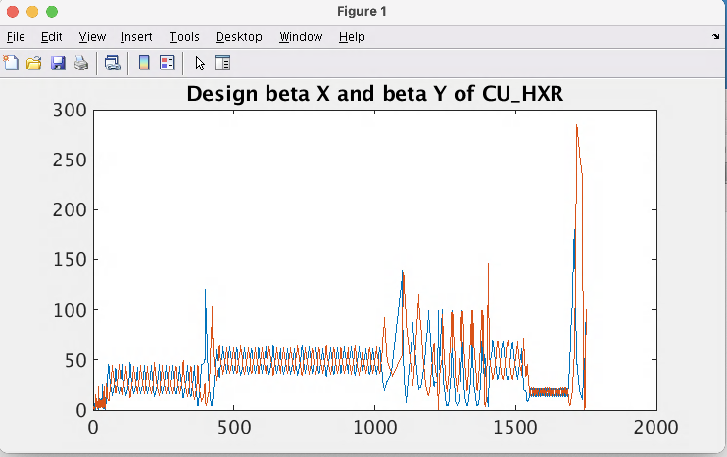
One can of course plot the columns to inspect beta, eta etc.
>> twiss_d=eget('BMAD:SYS0:1:CU_HXR:DESIGN:TWISS',{'provider','pva'});
>> plot(twiss_d.s, twiss_d.beta_x);
>> hold on
>> plot(twiss_d.s, twiss_d.beta_y);
>> title('Design beta X and beta Y of CU\_HXR');
In this example we retrive the DESIGN R-matrices of the SC_HXR beampath:
>> rmat_d=eget('BMAD:SYS0:1:SC_HXR:DESIGN:RMAT',{'provider','pva'});
Inspect first 10 rows of the table:
>> rmat_d([1:10],:)
Inspect all the element names (column element'):
>> rmat_d.element
One can extract the familiar 6x6 R-matrix of a given element by name, for instance 'SQ02B', by extracting the 36 columns 5 to 40, converting that from a 1 row table to array, and then array to 6x6 matrix (note the transpose operator at the end):
>> reshape(table2array(rmat_d(strcmp(rmat_d.element,'SQ02B'),5:40)),6,6)'

ans =

    1.0000    1.6270         0         0         0         0
         0    1.0000         0         0         0         0
         0         0    1.0000    1.6270         0         0
         0         0         0    1.0000         0         0
         0         0         0         0    1.0000    0.2703
         0         0         0         0         0    1.0000
One can retrieve data from the Oracle infrastructure database directly within Matlab. This uses an EPICS 7 service accessed via erpc (EPICS Remote Procedure Call):
Presently the service offers the following tables:
INFR:SYS0:1:BEAMPATHS    A 1 column table of names of beampaths in
                         LCLS complex, CU_HXR, SC_SXR etc

INFR:SYS0:1:CU_HXR       A table of the modelled devices in CU_HXR
INFR:SYS0:1:CU_SXR       A table of the modelled devices in CU_SXR
INFR:SYS0:1:SC_HXR       A table of the modelled devices in SC_HXR
INFR:SYS0:1:SC_SXR       A table of the modelled devices in SC_SXR
INFR:SYS0:1:SC_BSYD      A table of the modelled devices in SC_BYSD
INFR:SYS0:1:SC_DIAG0     A table of the modelled devices in SC_DIAG0
INFR:SYS0:1:SC_DASEL     A table of the modelled devices in SC_DASEL

INFR:SYS0:1:DEVICES      A table of all devices, both modelled (aka MAD) and
                         not modelled, in LCLS (> 6000 rows).
Access these tables using erpc, eg:
>>  sc_devices_js = erpc(nturi('INFR:SYS0:1:SC_SXR'));
>>  sc_devices_t=nttable2table(sc_devices_js);
>>  sc_devices_t(1:10,1:8)   % Display first 10 rows of table of SC_SXR elements

ans =

  10×8 table

      ELEMENT              DEVICE            KEYWORD       AREA      SECTOR      MODEL      SUML_M      LINACZ_M
    ____________    _____________________    ________    ________    _______    _______    _________    ________

    {'SOL1BKB' }    {'SOLN:GUNB:100'    }    {'SOLE'}    {'GUNB'}    {'S00'}    {'MAD'}    -0.071705    -10.116
    {'CATHODEB'}    {'CATH:GUNB:100'    }    {'INST'}    {'GUNB'}    {'S00'}    {'MAD'}            0    -10.045
    {'CQ01B'   }    {'QUAD:GUNB:212:1'  }    {'QUAD'}    {'GUNB'}    {'S00'}    {'MAD'}      0.24653    -9.7981
    {'SQ01B'   }    {'QUAD:GUNB:212:2'  }    {'QUAD'}    {'GUNB'}    {'S00'}    {'MAD'}      0.24653    -9.7981
    {'SOL1B'   }    {'SOLN:GUNB:212'    }    {'SOLE'}    {'GUNB'}    {'S00'}    {'MAD'}      0.24653    -9.7981
    {'VV01B'   }    {'- NO EPICS NAME -'}    {'INST'}    {'GUNB'}    {'S00'}    {'MAD'}      0.38748    -9.6572
    {'XC01B'   }    {'XCOR:GUNB:293'    }    {'XCOR'}    {'GUNB'}    {'S00'}    {'MAD'}       0.4845    -9.5602
    {'YC01B'   }    {'YCOR:GUNB:293'    }    {'YCOR'}    {'GUNB'}    {'S00'}    {'MAD'}       0.4845    -9.5602
    {'BPM1B'   }    {'BPMS:GUNB:314'    }    {'BPM' }    {'GUNB'}    {'S00'}    {'MAD'}      0.48965     -9.555
    {'IM01B'   }    {'TORO:GUNB:360'    }    {'IMON'}    {'GUNB'}    {'S00'}    {'MAD'}      0.59469      -9.45
Print just all element and device names (device name may be printed as summary, eg char [1×17]
>> sc_devices_t(:,{'ELEMENT','DEVICE'})
Print only device names:
>> sc_devices_t.DEVICE
See the unique list of AREAs, as defined by the Beamline Boundaries PRD:
>>  unique(sc_devices_t.AREA)

ans =

  22x1 cell array

    {'BC1B'  }
    {'BC2B'  }
    {'BSYS'  }
    {'BYP'   }
    {'COL0'  }
    {'COL1'  }
    {'DMPS_1'}
    {'DMPS_2'}
    {'DOG'   }
    {'EMIT2' }
    {'EXT'   }
    {'GUNB'  }
    {'HTR'   }
    {'L0B'   }
    {'L1B'   }
    {'L2B'   }
    {'L3B'   }
    {'LTUS'  }
    {'SLTS'  }
    {'SPD_1' }
    {'SPS'   }
    {'UNDS'  }
To see for instance only the rows for AREA L1B, one can select matching rows with strcmp:
>> sc_devices_t(strcmp(sc_devices_t.AREA,'L1B'),:)
The OPSTAT column of the table returned by the INFR:SYS0:1<beampath> PVs, like INFR:SYS0:1:SC_HXR, gives the controls commissioning status of the device. For instance, installed, wired, commissioned etc. OPSTAT is typically column 10. So, of the devices at the head of the machine (rows 1-10), the following is known by Oracle. At the time of writing May 2021, magnet like devices are reliably updated, but not others so far.
>> sc_devices_t(1:10,[1,2,3,10])

ans =

  10×4 table

      ELEMENT              DEVICE            KEYWORD              OPSTAT
    ____________    _____________________    ________    ________________________

    {'SOL1BKB' }    {'SOLN:GUNB:100'    }    {'SOLE'}    {'Not Installed'       }
    {'CATHODEB'}    {'CATH:GUNB:100'    }    {'INST'}    {' '                   }
    {'CQ01B'   }    {'QUAD:GUNB:212:1'  }    {'QUAD'}    {'Commissioned, Online'}
    {'SQ01B'   }    {'QUAD:GUNB:212:2'  }    {'QUAD'}    {'Commissioned, Online'}
    {'SOL1B'   }    {'SOLN:GUNB:212'    }    {'SOLE'}    {'Commissioned, Online'}
    {'VV01B'   }    {'- NO EPICS NAME -'}    {'INST'}    {' '                   }
    {'XC01B'   }    {'XCOR:GUNB:293'    }    {'XCOR'}    {'Commissioned, Online'}
    {'YC01B'   }    {'YCOR:GUNB:293'    }    {'YCOR'}    {'Commissioned, Online'}
    {'BPM1B'   }    {'BPMS:GUNB:314'    }    {'BPM' }    {' '                   }
    {'IM01B'   }    {'TORO:GUNB:360'    }    {'IMON'}    {' '                   }
An HLA cand then check potential devices for commissioning with constructs like the following. To check on a single device:
>> sc_devices_t(strcmp(sc_devices_t.DEVICE,'YCOR:GUNB:713'),10)

ans =

 table

            OPSTAT
   ________________________

   {'Commissioned, Online'}
To filter on commissioned-ness:
>> sc_devices_t(strcmp(sc_devices_t.OPSTAT,'Commissioned, Online'),2)

ans =

  5×1 table

         DEVICE
    ___________________

    {'QUAD:GUNB:212:1'}
    {'QUAD:GUNB:212:2'}
    {'SOLN:GUNB:212'  }
    {'XCOR:GUNB:293'  }
    {'YCOR:GUNB:293'  }
    {'XCOR:GUNB:388'  }
    {'YCOR:GUNB:388'  }
    …
The following programming pattern will make GUIs describe what happened when they encounter a problem, what they were in the middle of doing when the error occurred. It also makes the GUI display that information in a dialog box, and also print tall the relevant information to a log. In short, just use it everywhere. It works for GUIs as well as for functions and scripts called outside the context of a GUI.
When your code detects an error, immediately (on the next line after you detected the error) issue a message using the Matlab "error" function.
The error() function's first argument should be a message code string, in the Matlab style, using a prefix id specific to your app. You use the id in the callback function to identify your app's exceptions. This is important because your app's exceptions should not cause stacktraces in the log (the ugly and largely useless "crash" stuff). Only the others, ie matlab's own exceptions, should cause such stacktraces. In that way, errors like "division by 0" get a stacktrace, useful for debugging, whereas errors like "Couldn't move wire scan motor" do not, since that's not a bug in matlab, it's just something it wasn't able to do but handled gracefully.
In every GUI Callback function, use try/catch, with
uiwait(errordlg(lprintf())) in the catch block:
In every other (non-callback method), especially API methods, "throw exception." That
is, whenever the program can't go on because of a functional problem like you detect from
EPICS that a wire is stuck, call error(). The method SHOULD also
lprintf what happened.
[NOTE: constants below eg STDERR, WS_EXID_PREFIX etc, are defined in wirescan_const.m).
function scanWireName_pmu_Callback(hObject, eventdata, handles)
wirescan_const;
try
    scanWireInit(hObject,handles,get(hObject,'Value'));
catch ex
    if ~strncmp(ex.identifier,WS_EXID_PREFIX,3)
        fprintf(STDERR, '%s\n', getReport(ex,'extended'));
    end
    uiwait(errordlg(...
        lprintf(STDERR, 'Problem changing wire. %s', ex.message)));
end

function handles = scanWireInit(hObject, handles, wireId)
…
   initFWS(handles);   % API method can call other methods
   …
   function initFWS( handles )
      status = lcaPutSmart( pvName_reinit, initcode, 'short' );
      if ( status ~= LCA_SUCCESS )
         msgtext=lprintf(STDERR, 'Motor init failed', pvName_reinit );
         error('WS:MOTORINITFAILED', msgtext );
The message text SHOULD end in a period. The period is important because using the try catch scheme and using matlab's builtin argument processing, messages are chained together.
An example of issuing an error() and printing to the log in one line. Note that the message says what is wrong AND what a user might then do.
    error('EM:NOGOODDATAREMAINS', lprintf(STDOUT,...
        ['No data remaining that has both good measurement status' ...
           ' and user approved for use. Please include more scanned ' ...
           ' device setpoints (Quad values or wires), or check "Use"'...
           ' to allow inclusion of more in processing.']));
All CVS commands follow the keyword cvs.
To start working with CVS, you must check out a module (directory). This will put the files of that CVS module into your working directory. For example, make a working directory, cd to it, checkout the matlab/toolbox files, and cd down into the toolbox subdirectory where you'll find the matlab files:
$ mkdir work
$ cd work
$ cvs checkout matlab/toolbox
$ cd matlab/toolbox
Now you can make edits to the files, or create new ones.
Make sure all your scripts and functions include help at the top. Following the Matlab conventions for help comments will ensure that Matlab commands like "help" and "lookfor" will work properly.
You can update the files in your local directory with any changes made to them (by other people) in the repository.
$ cvs update -dA
If by chance someone else has also changed a file you have been working on, and they have committed their change before you did, then when you do the update CVS will attempt simply merge their changes into yours. The cvs update will be report that to you by printing the name of the file prefixed by "M", e.g.:
$ cvs update -dA
cvs update: Updating .
RCS file: /afs/slac/g/lcls/cvs/package/matlab/toolbox/lem.m,v
retrieving revision 1.4
retrieving revision 1.6
Merging differences between 1.4 and 1.6 into lem.m
M lem.m
If CVS was unable to automatically merge, you'll have a so-called "merge conflict".
There are guides on the interwebs to help you fix CVS conflicts; see for instance
. Basically, in the file that got a merge
conflict, look for lines between marker lines inserted by CVS that look like ">
> > > > > >" and "< < < < < < <
<". Hand edit the file to remove the marker lines and replace the lines so
marked with what you want. Then try the cvs update again.
If you created a new local file, you can register it with the CVS repository with "add". You have to also cvs commit it before it's really uploaded to the repository (see below).
$ cvs add hist2.m
If you want to remove a file from the CVS repository, remove it from your directory first, then tell CVS to remove it from the repository. By the way, CVS doesn't actually remove it, rather CVS puts removed files in a special subdirectory of the module named "Attic." For example see matlab/toolbox/Attic That way, it can recover and deliver previous versions of the file if they're checked out.
$ rm hist2.m
$ cvs remove hist2.m
Renaming a file in CVS involves copying the old file to its new name, cvs removing the old one, cvs adding the new one, and cvs committing both:
$ mv old new
$ cvs remove old
$ cvs add new
$ cvs commit -m "Renamed old to new" old new
Sometimes you want to know how your local files differ from the ones in the repository.
cvs diff hist2.m
After you made changes to a local file or directory of files (and tested them), you can upload the files back to the repository. This operation is called "commit". If you do the whole directory CVS will work out which ones changed and commit only those. NOTE: It's a very good idea to do a cvs update -dA immediately prior to attempting a cvs commit, to make sure that whatever you intend to commit hasn't already been changed in the repository by someone else since you did your cvs checkout.
$ cvs update -dA      Check for changes since your last checkout
$ cvs commit -m "this is what I did to the file" moments.m    or
$ cvs commit -m "the reason I changed all these files"
Some good guidelines for using CVS can be found at bib:cvsbestpractices.
It is important that the people involved with running the accelerator know of all software changes. It is especially important that any software which impacts accelerator operations in any way, particularly with respect to safety or to beam, is released in a controlled manner. It is also important to have a peer review before releasing code. Review can lead to more efficient and effective code and uncover potential problems that the developer may have missed. It leads to more effective collaboration among developers and helps to prevent code duplication. For these reasons, all production software in the control system of the SLAC Accelerator Complex, must be reviewed and released using the following procedure if it meets the threshold defined below.
Code review and formal release must take place for any deployment of production code totaling more than 300 new/modified lines. It must also take place for non-trivial changes even if the number of modified lines is less than this. Non-trivial changes typically include new functionality such as (but not limited to) the following:
An example of a trivial change would be a simple and specific bug fix or adding a simple UI element (like a logbook button); this does not require following the formal review/release procedures below. It is left to the developer to determine if their change is trivial and to ensure that they follow these rules if their change is non-trivial. It is also left to the developer and reviewer to determine what form code review takes and if any external tools are used (e.g. Github) to aid in the process. The reviewer may be anyone the developer chooses, and the proposed reviewer should be transparent about their availability/expertise while reserving the right to decline.
There is a writeup of Matlab Programming Standards that must be referenced as part of code review. This does not imply that all pre-existing code has to conform to the Matlab Programming Standards. Only the new or newly modified portions of the code are expected to conform to these standards. It is not specified how detailed the review has to be, this is intentionally left to the developer and the reviewer. At a minimum, the reviewer MUST verify the following for the new/modified code they are reviewing:
Code Review Procedure:
Code Release Procedure:
This completes the review and release procedure! Additional helpful information is listed below if you have questions:
For Matlab software, the mechanics of a software release (cvs commit and deployment), are given above.
This appendix describes the support for starting Matlab GUI apps from EPICS displays.
"xterm -iconic -T \"LiTrack GUI xterm\" -e MatlabGUI run_LiTrack_GUI"EPICS_CA_ADDR_LIST="lcls-prod01:5062
$EPICS_CA_ADDR_LIST" (so launched GUIs all use the lcls-prod01 gateway), and then
executes:
$ matlab -glnx86 -nosplash -nodesktop -r startLCLS,$1 -logfile $log_file
$ MatlabGUI <yourgui> [epics_max_array_size_specification]
The following are planned, but are not included in this version (Dec 11, 2019);