Throughput Time Series Patterns (Diurnal and Step Functions) Les Cottrell, Connie Logg IEPM-BW time series | Diurnal fits for: BBCP disk, BBCP memory, BBFTP, Iperf

IEPM Home Page  IEPM Site Map  Network Monitoring  PingER  IEPM-BW Home IEPM Papers and Presentations

Description

The achievable iperf TCP throughputs seen in Fig. 1 vary by more than a factor of 10 from site to site.

Figure 1: Logical routes to the remote IEPM-BW sites (October 2002).  shows the logical routes from SLAC. The boxes with bold outlines are monitoring sites in their own right. The labels in italics in boxes indicate the host has a 100Mbit/s connection. Other hosts have Gbits/s connections. The box shading indicates the participant type. Diagonal lines are for PPDG/GriPhyN/HENP collaborators, hashed shading indicates the site is a network measurement collaborator, and the un-shaded boxes are for European Data Grid collaborators. The clouds are for Internet Service providers (ISPs). The grey lettering in the clouds indicates the "GigaPoP" (e.g. ATL means Atlanta). The numbers by the sites indicate the average measured throughput from August 24 through October 26, 2002. For the measurements reported SLAC had OC12 (622Mbps) connections to ESnet and Internet2.

By design, hosts with 1000GE NICs had higher speed connections (typically 622Mbits/s) to the Internet and, as expected, higher performance is observed. By using large windows and multiple streams we were able to measure throughputs of  several hundreds of Mbits/s across both transcontinental and transoceanic links.

Viewing our time series plots of the throughputs, we observe two major types of behavior that may overlap at times.

1.       Sudden step changes in throughput. These are usually associated with a network change, e.g. a new route, or a link upgrade. They may also be associated with a remote host change, e.g. a new CPU or a change in the Network Interface Card (NIC) used.

Figure 2: Time series of iperf TCP and other throughputs measured from SLAC to CERN for 28 days starting Nov 2, 2002. Also shown are the ping minimum as grey bars and average Round Trip Times (RTT) as red bars.

2.       Oscillations in the throughput on a daily basis, e.g. high throughput at night or weekends when there is lower utilization and congestion, and higher performance at other periods. We refer to the daily changes as diurnal variations.

Figure 3: Time series of iperf and other throughputs from SLAC to Caltech for 28 days starting Nov 2, 2002.

If the time series are fairly flat (e.g. there are only small diurnal changes) then sudden changes in throughput show up as multimodal peaks in histograms of the throughput (see Fig. 4). They also show up in the moving averages with large relative standard deviations for the set of points close to the change.

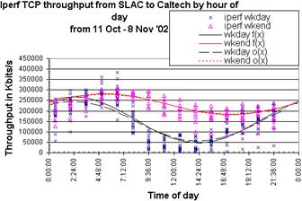
Fig 4: Histogram of the iperf TCP throughputs for Fig. 3. The red line shows the Cumulative Distribution Function  (CDF).

About 25% of the remote hosts exhibit large diurnal variations.. For such hosts we use a simple fit to:

f(x) = abs(a) * sin(x + b) + c

where x = time of day (in radians, i.e. start of day = 0, end of day = 2 * pi). We use as the least-squares fit starting values, c = average throughput, a = standard deviation of throughput, and c = pi/2. This fit enables an easy characterization of the diurnal variability. The fitting can be further simplified, by noting that b (the phase angle) should stay fairly constant for a given site (if there is a diurnal variation then the busy/congested periods are likely to be the same from weekday to weekday). Fig 5 shows a least-squares fit to iperf TCP data measured from SLAC to Caltech from October 11 to November 8, 2002, where the x axis is the time of day of the measurement, and the weekday measurements have been separated from the weekend measurements. Also shown are the curves (dashed lines) from simply using the starting values for a and c, and leaving b at the value found in the fit. It can be seen that we can do almost as good with the simple fit, and not have to resort to least-square fitting techniques. The difference in the fitted value and initial estimate can be expressed as diff = abs((fit-initial)/fit) and yields median values (for 39 remote hosts) of < 2% for a and  6% for b. Since a and c are simple to estimate from the data, and b should stay roughly constant for a given site, this proves to be a simple method for quantifying the diurnal nature of the data.

We have found that we can roughly quantify the "diurnalness" of the data for a given node by looking at the error on the fit parameter b (db). In essence, db determines how the diurnal nature of the data is clearly defined to allow b to be well determined. Values of db of < 0.2 appear to indicate candidates for paths with large diurnal variations. We identify these large diurnal variations by eyeball by looking at a plot such as shown in Fig. 5.  For Fig. 5 the values of db are 0.04 (weekday) and 0.1 (weekend). Current examples can be found in Master Diurnal fit for iperf.sum.

As expected, there is usually different and less diurnal variation for weekend data.  We are looking at ways to fold the diurnal variations into the predictions, for example by predicting the value at some time, from the value at the same time a week ago.  Though this may be less accurate than a prediction from more recent data, it may be of value if there is no recent data.

Figure 5: Iperf TCP diurnal variations. Weekdays in blue, weekends in magenta. The fits are to sin functions.