Hands on 3: Build detector, retrieve simulation results
In this third hands-on you will learn how to:
- Create a semi-realistic geometry
- Collect simulation output from sensitive detectors in hits
- Use the event user-action to dump event information from hits on screen
The code for this hands-on session
is here (
for your reference, the complete solution
is also availavble here).
Copy the the tar ball to your local area.
Follow the instructions of Hands On
1 to configure with cmake the code and build it. Try
out the application:
  $ cd <tutorial>

  $ tar xzf HandsOn3.tar.gz

  $ cd HandsOn3

  $ cmake .

  $ make -j 2 -f Makefile

  $ ./SLACtut
|
Note: Ignore compiler warning messages. They disappear once you complete the exercise.
This geometry should be displayed:
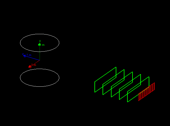
The geometry is same as Hands On
2, as we will start from here to build a two-arm spectrometer. The first arm
is already defined, and in the first exercise you will build
the second arm completed with a calorimeter:
- Each arm includes 5 drift-chamber planes to measure the
position of the passing particles (in green).
- Each arm includes a hodoscope made of scintillator plates to
measure the time-of-flight of the incoming particles (in red).
- A central magnetic system to deflect the charged particles
(white cylinder).
- Exercise: An electromagnetic calorimeter composed of CsI crystals
(yellow in the picture).
- Exercise: An hadronic sampling calorimeter composed of Lead as
absorber and Scintillator as active material (blue).
The second arm can be rotated between runs. The
magnetic-field value can also be changed. User defined UI commands allow
to change arm rotation and magnetic field value at run time.
At the end of this hands on the complete geometry will look
like:
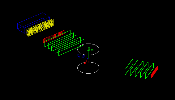
There are 6 steps involved in this exercise to build the geometry.
The
application will compile and work correctly only when the first 5
steps are completed (however it is a good idea to try to compile at
each step to fix early trivial errors).
The last step is optional because it has the goal
to change visualization attributes (colors of geometry elements) and
has no effect on simulation results.
Reminder on different ways to create a geometry setup:
- After creating solids and logical volumes you can place physical volumes
via
G4PVPlacement (these have been already covered in Hands On 2).
- You you can place multiple copies of the same logical volumes via
multiple placements.
- Or you can use of
G4PVParametrised to place multiple copies
of the same volume with dimensions/position parametrised
by the copy number.
- You can also use replicas to slice a larger volume in smaller
pieces.
Check the DetectorConstruction.hh file, since many
variables you will need are already defined there.
Implement the second hodoscope.
The second hodoscope is composed of 25 planes of dimensions:
10x40x1 cm. The hodoscopes tiles are composed of scintillator material.
Instantiate
a single shape and a single logical volume. Place 25 physical volume placements
in the second arm mother volume (this mother volume is already created).
Each tile is positioned at Y=Z=0 with
respect to the mother volume, while the X coordinates depends on the
tile numnber.
Hint: Check what is done for the hodoscope of the first
arm. Remember dimensions passed to Geant4 solid classes are half
dimensions.
Solution
| DetectorConstruction.cc File: |
      // =============================================

  // Exercise 1

     // Complete the full geometry.

     // Note that second arm, by default is rotated of

     // 30 deg.

     // Step 1: Add an hodoscope with dimensions (X,Y,Z):

     //         (10,40,1)cm made of scintillator.

     //         There are 25 planes placed at Y=Z=0 (w.r.t. mother volume)

     // hodoscopes in second arm

     G4VSolid* hodoscope2Solid = new G4Box("hodoscope2Box",5.*cm,20.*cm,0.5*cm);

     fHodoscope2Logical = new G4LogicalVolume(hodoscope2Solid,scintillator,"hodoscope2Logical");

     for (G4int i=0;i<25;i++)

     {

           G4double x2 = (i-12)*10.*cm;

           new G4PVPlacement(0,G4ThreeVector(x2,0.,0.),fHodoscope2Logical,"hodoscope2Physical",secondArmLogical,false,i,checkOverlaps);

     }
|
Build the drift chambers.
The second arm contains 5 drift chambers made of argon gas with
dimensions 300x60x2 cm. These are equally spaced inside the second arm
starting from -2.5 m to -0.5 m along the Z coordinate.
Hint: Use same methods used for step 1.
Solution
| DetectorConstruction.cc File: |
      // Step 2: Add 5 drift chambers made of argon, with dimensions (X,Y,Z):

     //         (300,60,2)cm

     //         These are placed equidistant inside the second arm at distances from -2.5m

     //         to -0.5m

     // drift chambers in second arm

     G4VSolid* chamber2Solid = new G4Box("chamber2Box",1.5*m,30.*cm,1.*cm);

     G4LogicalVolume* chamber2Logical = new G4LogicalVolume(chamber2Solid,argonGas,"chamber2Logical");

     for (G4int i=0;i<5;i++)

     {

           G4double z2 = (i-2)*0.5*m - 1.5*m;

           new G4PVPlacement(0,G4ThreeVector(0.,0.,z2),chamber2Logical,"chamber2Physical",secondArmLogical,false,i,checkOverlaps);

     }
|
Add a virtual wire plane in the drift chambers.
Add a plane of wires in the drift chambers of step
2. To simplify our problem we do not describe the single wires,
instead we add a new argon-filled volume of dimensions 300x60x0.02 cm
in the center of each of the five drift chambers.
This exercise is technically simple (a single placement), however it
shows a very useful concept: we create a single instance of this
volume and we place it once inside the mother logical volume (the
drift chamber logical volume), since the mother volume is repeated
five times, each chamber gets its own wire plane. We are
reducing the number of class instances needed for the description
of our geometry (and thus reducing the memory footprint of our
application, beside making the code more compact and readable).
Solution
| DetectorConstruction.cc File: |
     // Step 3: Add a virtual wire plane of (300,60,0.02)cm

     //         at (0,0,0) in the drift chamber

     // virtual wire plane

     G4VSolid* wirePlane2Solid  = new G4Box("wirePlane2Box",1.5*m,30.*cm,0.1*mm);

     fWirePlane2Logical = new G4LogicalVolume(wirePlane2Solid,argonGas,"wirePlane2Logical");

     new G4PVPlacement(0,G4ThreeVector(0.,0.,0.),fWirePlane2Logical, "wirePlane2Physical",chamber2Logical,false,0,checkOverlaps);
|
Build an electromagnetic calorimeter.
An electromagnetic calorimeter has the goal to measure the energy
of absorbed particles. Its dimensions are such that an electron or
gamma of the typical beam energy is fully absorbed, while hadrons
(such as protons), only leave a fraction of their
energy in an electromagnetic calorimeter (because it is too
short). In our example we implement a homogeneous calorimeter made of
a matrix of CsI
crystals (a charged particles emits light when interacting with this
material, the quantity of light produced is proportional to the
energy lost by the particle).
Build a 300x60x30 cm CsI calorimeter. The calorimeter is made of a
matrix of 15x15x30 cm crystals. Instead of using placements we show
how to use parametrised solids. The idea is that the position of the
placement is a function of the crystal number. The parametrization
class is already available for you in
CellParametrisation. Check the method
CellParameterisation::ComputeTransformation(...) to
understand how the calorimeter cells are implemented.
The calorimeter should be placed at 2 m downstream along Z in the second arm
mother volume.
Solution
| DetectorConstruction.cc File: |
      // Step 4: Build CsI EM-calorimeter of (300,60,30)cm

     //         placed at (0,0,2)m in the second arm.

     //         The calorimeter is made of 80 cells,

     //         parametrised according to CellParametrisation

     //         G4VPVParameterisation concrete instance.

     //         This class parametrize the position of each cell depending

     //         on its copy number.

     //         The cells have dimensions 15x15x30 cm.

     //         (you could use placements or replicas, but here

     //         we show how to use parametrisations to build geometry)

     // CsI calorimeter

     G4VSolid* emCalorimeterSolid = new G4Box("EMcalorimeterBox",1.5*m,30.*cm,15.*cm);

     G4LogicalVolume* emCalorimeterLogical = new G4LogicalVolume(emCalorimeterSolid,csI,"EMcalorimeterLogical");

     new G4PVPlacement(0,G4ThreeVector(0.,0.,2.*m),emCalorimeterLogical,"EMcalorimeterPhysical",secondArmLogical,false,0,checkOverlaps);


     // EMcalorimeter cells

     G4VSolid* cellSolid = new G4Box("cellBox",7.5*cm,7.5*cm,15.*cm);

     fCellLogical = new G4LogicalVolume(cellSolid,csI,"cellLogical");

     G4VPVParameterisation* cellParam = new CellParameterisation();

     new G4PVParameterised("cellPhysical",fCellLogical,emCalorimeterLogical,kXAxis,80,cellParam);
|
Implement the hadronic calorimeter
This is a sampling calorimeter made of lead as absorber material
(used for its high density) interleaved with plates of scintillator
(the active material). It is called sampling because only a fraction of
the energy lost by the particles is measured (the one lost in the
active material), this is proportional to the total energy
loss and hence to the impinging particle energy (you may be aware of
the problem of non-compensation, but we will not discuss it
here).
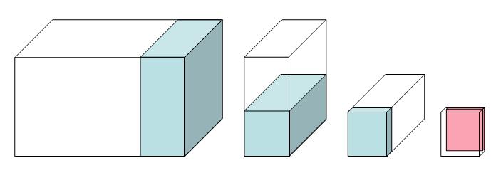
Implement the calorimeter using replicas to slice a larger volume into
smaller units. Each cell has 20 layers of 4 cm thick lead plate and 1 cm
thick scintillator plate. The size of the plate is 30 cm square. The
calorimeter has 10 towers of 2 cells each. Here is a
schematic drawing of the calorimeter. From left to right: the full
calorimeter with a single tower;
a single tower is divided in two cells; the third picture shows a single
cell
with a single layer; finally a single layer with the active scintillator tile.
Beam is perpendicular to the screen.
-
The whole Hadronic calorimeter box is made of lead. The size is 3 m in
width, 60 cm in height, and 1 m in depth. It should be placed 3 m
downstream inside the second arm.
-
Replica is defined along one Cartesian axis, define
a tower of 30 cm width. It is also made of lead.
The height and depth of this column are equal to
the full calorimeter dimensions.
-
A cell made of lead has half height of a tower.
-
Each layer in a cell is 5 cm thick. It is made of lead as well.
-
Finally a scintillator tile should be placed inside each layer.
You can now test the setup, use UI commands
/tutorial/detector/armAngle,
/tutorial/field/value to move the second arm and set the
magnetic field. Note that geometry can be changed only between
runs. The methods DefineCommands gives an example on how
to define application specific commands (this is an advanced topic not
discussed in this Hands-On's). Use the
help UI command to get help on commands.
Solution
| DetectorConstruction.cc File: |
     // Step 5: Add a "sandwich" hadronic calorimeter of dimensions:

     //         (300,60,100)cm.

     //         The calorimeter absorber is made of lead. It is divided in

     //         towers of (30,60,100)cm. Use replica along X-axis

     //         for towers.

     //         A tower is composed of cells, "stacked" along Y-axis

     //         Each cell has dimension (30,30,100)cm.

     //         A cells has "layers" along Z-axis. Each layer has dimensions

     //         (30,30,5)cm. Also in this case use replicas.

     //         Finally in each layer there is a tile of scintillator material

     //         of dimensions (30,30,1)cm

     // hadron calorimeter

     G4VSolid* hadCalorimeterSolid = new G4Box("HadCalorimeterBox",1.5*m,30.*cm,50.*cm);

     G4LogicalVolume* hadCalorimeterLogical = new G4LogicalVolume(hadCalorimeterSolid,lead,"HadCalorimeterLogical");

     new G4PVPlacement(0,G4ThreeVector(0.,0.,3.*m),hadCalorimeterLogical,"HadCalorimeterPhysical",secondArmLogical,false,0,checkOverlaps);


     // hadron calorimeter column

     G4VSolid* HadCalColumnSolid = new G4Box("HadCalColumnBox",15.*cm,30.*cm,50.*cm);

     G4LogicalVolume* HadCalColumnLogical = new G4LogicalVolume(HadCalColumnSolid,lead,"HadCalColumnLogical");

     new G4PVReplica("HadCalColumnPhysical",HadCalColumnLogical,hadCalorimeterLogical,kXAxis,10,30.*cm);


     // hadron calorimeter cell

     G4VSolid* HadCalCellSolid = new G4Box("HadCalCellBox",15.*cm,15.*cm,50.*cm);

     G4LogicalVolume* HadCalCellLogical = new G4LogicalVolume(HadCalCellSolid,lead,"HadCalCellLogical");

     new G4PVReplica("HadCalCellPhysical",HadCalCellLogical,HadCalColumnLogical,kYAxis,2,30.*cm);


     // hadron calorimeter layers

     G4VSolid* HadCalLayerSolid = new G4Box("HadCalLayerBox",15.*cm,15.*cm,2.5*cm);

     G4LogicalVolume* HadCalLayerLogical = new G4LogicalVolume(HadCalLayerSolid,lead,"HadCalLayerLogical");

     new G4PVReplica("HadCalLayerPhysical",HadCalLayerLogical,HadCalCellLogical,kZAxis,20,5.*cm);


     // scintillator plates

     G4VSolid* HadCalScintiSolid = new G4Box("HadCalScintiBox",15.*cm,15.*cm,0.5*cm);

     fHadCalScintiLogical = new G4LogicalVolume(HadCalScintiSolid,scintillator,"HadCalScintiLogical");

     new G4PVPlacement(0,G4ThreeVector(0.,0.,2.*cm),fHadCalScintiLogical,"HadCalScintiPhysical",HadCalLayerLogical,false,0,checkOverlaps);
|
Provide visualization attributes for the second arm volumes.
Note
that hadronic calorimeter sub-structure is by default made invisible to reduce
visual clutter. This is helpful to hide the geometry details less important
to the simulation.
Solution
| DetectorConstruction File: |
     // visualization attributes ------------------------------------------------

     // Step 6: uncomment visualization attributes of the newly created volumes

     G4VisAttributes* visAttributes = new G4VisAttributes(G4Colour(1.0,1.0,1.0));

     visAttributes->SetVisibility(false);

     worldLogical->SetVisAttributes(visAttributes);

     fVisAttributes.push_back(visAttributes);


     visAttributes = new G4VisAttributes(G4Colour(0.9,0.9,0.9));   // LightGray

     fMagneticLogical->SetVisAttributes(visAttributes);

     fVisAttributes.push_back(visAttributes);


     visAttributes = new G4VisAttributes(G4Colour(1.0,1.0,1.0));

     visAttributes->SetVisibility(false);

     firstArmLogical->SetVisAttributes(visAttributes);

     secondArmLogical->SetVisAttributes(visAttributes);

     fVisAttributes.push_back(visAttributes);


     visAttributes = new G4VisAttributes(G4Colour(0.8888,0.0,0.0));

     fHodoscope1Logical->SetVisAttributes(visAttributes);

     fHodoscope2Logical->SetVisAttributes(visAttributes);

     fVisAttributes.push_back(visAttributes);


     visAttributes = new G4VisAttributes(G4Colour(0.0,1.0,0.0));

     chamber1Logical->SetVisAttributes(visAttributes);

     chamber2Logical->SetVisAttributes(visAttributes);

     fVisAttributes.push_back(visAttributes);


     visAttributes = new G4VisAttributes(G4Colour(0.0,0.8888,0.0));

     visAttributes->SetVisibility(false);

     fWirePlane1Logical->SetVisAttributes(visAttributes);

     fWirePlane2Logical->SetVisAttributes(visAttributes);

     fVisAttributes.push_back(visAttributes);


     visAttributes = new G4VisAttributes(G4Colour(0.8888,0.8888,0.0));

     visAttributes->SetVisibility(false);

     emCalorimeterLogical->SetVisAttributes(visAttributes);

     fVisAttributes.push_back(visAttributes);


     visAttributes = new G4VisAttributes(G4Colour(0.9,0.9,0.0));

     fCellLogical->SetVisAttributes(visAttributes);

     fVisAttributes.push_back(visAttributes);


     visAttributes = new G4VisAttributes(G4Colour(0.0, 0.0, 0.9));

     hadCalorimeterLogical->SetVisAttributes(visAttributes);

     fVisAttributes.push_back(visAttributes);


     visAttributes = new G4VisAttributes(G4Colour(0.0, 0.0, 0.9));

     visAttributes->SetVisibility(false);

     HadCalColumnLogical->SetVisAttributes(visAttributes);

     HadCalCellLogical->SetVisAttributes(visAttributes);

     HadCalLayerLogical->SetVisAttributes(visAttributes);

     fHadCalScintiLogical->SetVisAttributes(visAttributes);

     fVisAttributes.push_back(visAttributes);
|
In this exercise we will cover basic aspects of retrieving
physics quantities from the simulation kernel.
The basic simulation output is called
hit (a user-defined class inheriting from G4VHit):
an energy deposit in space and time. Typically we are not
interested in hits in all detector elements, but instead we want to
retrieve information only for the relevant detector
components, to simulate the detector read-out (e.g. the scintillator tiles
in the hadronic calorimeter, and not the lead absorber).
In Geant4 this is achieved with the concepts of hits and
sensitive detectors (SD): you can attach a SD (a user class
inheriting from G4VSensitiveDetector) to a logical
volume, in this way Geant4 will call your user-code when a particle is
tracked in this specific volume. Information can be retrieved from the
G4Step (e.g. energy
deposited along the step) and a new hit is created (or an
existing hit is updated). Geant4 will keep track of all hits created
in the application. These can be retrieved at the end of the event for further
post-processing and writing to output.
We will show how to measure a quantity, for each event,
from the hodoscopes. The goal is to measure at what time and in which hodoscope
tile there was a hit.
The exercise is divided in three parts, and you will have to modify
four files:
HodoscopeHit.hh and HodoscopeHit.cc files
implement the hit class for the hodoscope.HodoscopeSD.cc implements the hodoscope sensitive
detector.DetectorConstruction.cc instantiates the sensitive detector
and attaches it to the correct logical volume.
Create a hit class.
This concrete Hit class represents a data container for only two
quantities: an integer value, representing the index of the hodoscope tile
that fired; and a double value, representing the time in which the
hodoscope tile fired. Reminder: a hodoscope is a simple set of
scintillators that measure the time in which a charged particle
passes through it. It can be used to performed time-of-flight
measurement and coarse-granularity position measurements.
You will need to modify the HodoscopeHit class. The class skeleton is
already prepared, you should add two data members that identify which hodoscope
tile has fired and register the time of the hit.
Note, that empty Constructor, the operators new and delete have been already
implemented. You should remove the empty implementation and
implement the correct methods. Implement/modify the Print method to dump
the hit content.
Important note on operator new and
operator delete: hits can put some
pressure on CPU, because, for each event, many hits may be created
and deleted at the end of the
event. Allocating on the heap is a
(relatively) CPU-intensive operation, thus the handling of hits may
cause some
performance degradation in a complex application.
To mitigate this we
use an allocator that allows for an efficient re-use memory and
avoid many calls to new/delete.
The first time a hit is created a memory pool is created that can hold
(like in an array) many hits. Each time a hit is created
with new operator we first look in this pool for an available
pre-allocated memory location. If an empty slot is available, we
re-use it, otherwise we grow the pool to contain more
hits.
With this technique we reduce substantially the new/delete cycles needed
for the simulation.
An additional complication is that in multi-threading
environments special attention is needed for the use of allocators.
We recognize this is an advanced topic that requires some
more advanced knowledge of C++. If you do not feel
comfortable with this discussion, you can remove from the HodoscopeHit.hh file
the lines defining the new and delete operators, the application will
work perfectly and since the hits are very simple and the simulation
program is not too complex you will not see any CPU penalty.
This exercise implements a single sensitive detector and one hit
type. In Hands On 4 additional
sensitive detectors are used with hits in the drift chambers and in
the calorimeters. You can study that code to see additional types
of hits (calorimeter hits are of some interest since accumulate energy
from several steps instead of creating a new hit at each step).
Solution
| HodoscopeHit.hh file: |
class HodoscopeHit : public G4VHit

 {

 public:

     HodoscopeHit(G4int i,G4double t);

     virtual ~HodoscopeHit() {}


     inline void *operator new(size_t);

     inline void operator delete(void*aHit);


     void Print();


     G4int GetID() const { return fId; }


     void SetTime(G4double val) { fTime = val; }

     G4double GetTime() const { return fTime; }


 private:

     G4int fId;

     G4double fTime;

};


 typedef G4THitsCollection<HodoscopeHit> HodoscopeHitsCollection;


 extern G4ThreadLocal G4Allocator<HodoscopeHit>* HodoscopeHitAllocator;


 inline void* HodoscopeHit::operator new(size_t)

 {

       if (!HodoscopeHitAllocator)

             HodoscopeHitAllocator = new G4Allocator<HodoscopeHit>;

       return (void*)HodoscopeHitAllocator->MallocSingle();

 }


 inline void HodoscopeHit::operator delete(void*aHit)

 {

       HodoscopeHitAllocator->FreeSingle((HodoscopeHit*) aHit);

 }
|
| HodoscopeHit.cc file: |
 G4ThreadLocal G4Allocator<HodoscopeHit>* HodoscopeHitAllocator;


 HodoscopeHit::HodoscopeHit(G4int i,G4double t)

 : G4VHit(), fId(i), fTime(t)

 {}


 void HodoscopeHit::Print()

 {

       G4cout << "  Hodoscope[" << fId << "] " << fTime/ns << " (nsec)" << G4endl;

 }
|
Create and manipulate hodoscope hits.
For this exercise you will modify HodoscopeSD.cc file.
Some part of
the code is already implemented, in particular the
initialization of the hits collection, use this code as a reference
for your future applications: it is important to understand the details of
how the registering of
hits with the Geant4 kernel works.
What you need to do for this exercise is to modify the method
ProcessHits and implement the logic to extract time and
position. This is the method that Genat4 kernel will call every time a
particle passes through the volume associated with this SD. The
G4Step object encodes the information regarding the
simulation step in the geometry volume.
Hint 1: Given a G4Step two points are defined
(G4StepPoint) that delimit the step itself (pre- and post-).
From each
point you can retrieve which volume the step belongs to via the
touchable history:
G4TouchableHistory* touchable = static_cast<G4TouchableHistory*>(
stepPoint->GetTouchable() );

G4int copyNumber = touchable->GetVolume()->GetCopyNo();
|
These two lines allows you to get the copy number of the volume
touched by the step (in our case the copy number for the hodoscope is
the tile number, see file DetectorConstruction.cc).
Hint 2: There are two G4StepPoint
defining a G4Step, which one of the two should you use,
pre- or post- step point? Why? The answer to this question is one of
the most trickiest part of Geant4 for a new user, be sure to
understand the reason why the two points are not equivalent!
Hint 3: We are simulating a scintillator detector that will
trigger only if some energy has been deposited (i.e. via ionization),
for example if a neutron passes through the detector (without making
interactions) its passage should not be recorded. Check the energy
deposited in the step, if zero do not do anything.
Hint 4: More than one step can be done by the same particle in
a single volume (why?), in addition secondaries produced in the volume
will also make steps in the SD. This mean that for a given primary particle we
can have more than one call to the ProcessHits.
A realistic detector electronics will responds with a
single measurement: to simulate this behavior every time a new step is
processed we check if the hit for the hodoscope tile that fired already
exists, if so we update the time information if the new hit happens
earlier than the already recorded one.
Solution
| HodoscopeSD.cc file: |
 G4bool HodoscopeSD::ProcessHits(G4Step* step, G4TouchableHistory*)

 {

       G4double edep = step->GetTotalEnergyDeposit();

       if (edep==0.) return true;


       G4StepPoint* preStepPoint = step->GetPreStepPoint();


       G4TouchableHistory* touchable = (G4TouchableHistory*)(preStepPoint->GetTouchable());

       G4int copyNo = touchable->GetVolume()->GetCopyNo();

       G4double hitTime = preStepPoint->GetGlobalTime();


       // check if this finger already has a hit

       G4int ix = -1;

       for (G4int i=0;i<fHitsCollection->entries();i++)

       {

             if ((*fHitsCollection)[i]->GetID()==copyNo)

             {

                  ix = i;

                   break;

             }

      }


       if (ix>=0) // if it has, then take the earlier time

       {

             if ((*fHitsCollection)[ix]->GetTime()>hitTime)

             { (*fHitsCollection)[ix]->SetTime(hitTime); }

       }

       else // if not, create a new hit and set it to the collection

       {

             HodoscopeHit* hit = new HodoscopeHit(copyNo,hitTime);

             fHitsCollection->insert(hit);

       }

       return true;

 }
|
Construct the SD and attach it to the correct logical volume.
We can now create an instance of the HodoscopeSD and attach it
to the correct logical volume. Add a separate instance of the SD to
each arm hodoscope. Give the names "/hodoscope1" and "/hodoscope2" to
these SDs. The same class is used for two logical volumes, the
two instances are recognized by Geant4 only via their names.
We are going to modify the method
ConstructSDandField in the DetectorCostruction class.
If you are already a user of older version of Geant4
(up to version 9.6) this is one of the new
main features introduced in version 10.0 to be compatible with multi-threading.
To reduce memory consumption geometry is
shared among threads, but sensitive-detectors are not.
Solution
| DetectorConstruction.cc file: |
 void DetectorConstruction::ConstructSDandField()

 {

     // sensitive detectors -----------------------------------------------------

     G4SDManager* SDman = G4SDManager::GetSDMpointer();

     G4String SDname;


     G4VSensitiveDetector* hodoscope1 = new HodoscopeSD(SDname="/hodoscope1");

     SDman->AddNewDetector(hodoscope1);

     fHodoscope1Logical->SetSensitiveDetector(hodoscope1);


     G4VSensitiveDetector* hodoscope2 = new HodoscopeSD(SDname="/hodoscope2");

     SDman->AddNewDetector(hodoscope2);

     fHodoscope2Logical->SetSensitiveDetector(hodoscope2);


     // magnetic field ----------------------------------------------------------

     fMagneticField = new MagneticField();

     fFieldMgr = new G4FieldManager();

     fFieldMgr->SetDetectorField(fMagneticField);

     fFieldMgr->CreateChordFinder(fMagneticField);

     G4bool forceToAllDaughters = true;

     fMagneticLogical->SetFieldManager(fFieldMgr, forceToAllDaughters);


 }
|
In this exercise we modify one of the user-actions to print on
screen the information collected from hodoscopes at the end of each event.
User actions allow to interact with the simulation to retrieve and
control the simulation results at specific points during the simulation of a run.
Different user action provides
specific interfaces to control the different aspects of the simulation. For
example, the G4UserEventAction class provides interfaces
to interact with Geant4 at the beginning and at the end of each
event. G4UserRunAction allows for the creation of a user-custom
G4Run object and it executes user-code at the beginning and at the
end of a run (this will be covered in the Hands On
4). G4VUserPrimaryGeneratorAction controls the
creation of primaries, G4UserSteppingAction allows to
retrieve information at each step (indipendentely of sensitive detectors), G4UserTrackingAction
allows for interaction with each G4Track and finally
G4UserStackingAction allows to control the urgency of
each new G4Track (advanced).
Note for users of older versions of Geant4:
Multi-threading requires user actions to be thread-private (differently
from initialization classes that are shared among threads). A new user initialization class is available in
version 10: G4VUserActionInitialization this provides a
method Build() in which all user actions are instantiated
(this method is called by each worker thread). A second method
BuildForMaster is called by the master thread. Among all
user actions the G4UserRunAction is the only one that can
also be instantiated for the master
thread, this is to allow for reduction
of results from worker threads to master thread
(e.g. sum the partial results of each thread into a global
result). This will be covered in the Hands On 4.
Using a G4UserEventAction print on screen the number
of hits and the time registered in the hodoscopes.
For this exercise you will need to modify in file EventAction.cc
the method EndOfEventAction, this method is called by
Geant4 at the end of the simulation of each event. The pointer to the
current G4Event is passed to the user-code. From this
object you will retrieve the hits collections for the two
hodoscopes and dump to screen the collected information.
Part of the EventAction code is already implemented.
In particular take a moment to study the method
BeginOfEventAction: in this method we retrieve the IDs of
the two collections. Note the if statement that allows
for an efficient search of the IDs, given the collection names, only
once. Searching with strings is a time consuming operation, this
method allows for reducing the CPU time, if many collections are
created this is an important optimization to consider.
Important: The code assumes you have called the two SDs:
"/hodoscope1" and "/hodoscope2" and that they create a hit collection
called "hodosopeColl". Change these if you have modified the names.
The EventAction is instantiated in the
ActionInitialization class. Take a look at it and see how
the EventAction is created.
The solution shows how to introduce some run-time checks of the
effective existence of the hits. While this is not necessary in this
simple code, this is a good code practice:
in large applications the presence of hits collections may be
decided at run time depending on the job configuration.
Solution
| EventAction.cc file: |
 void EventAction::EndOfEventAction(const G4Event* event)

 {

     // =============================================

     // Exercise 3

     // Print on screen the hits of the hodoscope

     // Step 1: Get the hits collection of this event

     G4HCofThisEvent* hce = event->GetHCofThisEvent();

     if (!hce)

     {

           G4ExceptionDescription msg;

           msg << "No hits collection of this event found.\n";

           G4Exception("EventAction::EndOfEventAction()","Code001", JustWarning, msg);

           return;

     }

     // Step 2: Using the memorised IDs get the collections

     // corresponding to the two hodoscopes

     // Get hits collections

     HodoscopeHitsCollection* hHC1 = static_cast<HodoscopeHitsCollection*>(hce->GetHC(fHHC1ID));

     HodoscopeHitsCollection* hHC2 = static_cast<HodoscopeHitsCollection*>(hce->GetHC(fHHC2ID));

     if ( (!hHC1) || (!hHC2)  )

     {

           G4ExceptionDescription msg;

           msg << "Some of hits collections of this event not found.\n";

           G4Exception("EventAction::EndOfEventAction()","Code001", JustWarning, msg);

           return;

     }

     //

     // Print diagnostics

     //

     G4int printModulo = G4RunManager::GetRunManager()->GetPrintProgress();

     if ( printModulo==0 || event->GetEventID() % printModulo != 0) return;


     G4PrimaryParticle* primary = event->GetPrimaryVertex(0)->GetPrimary(0);

     G4cout << G4endl

              << ">>> Event " << event->GetEventID() << " >>> Simulation truth : "

              << primary->GetG4code()->GetParticleName()

              << " " << primary->GetMomentum() << G4endl;


     // Step 3: Loop on the two collections and dump on screen hits

     // Hodoscope 1

     G4int n_hit = hHC1->entries();

     G4cout << "Hodoscope 1 has " << n_hit << " hits." << G4endl;

     for (G4int i=0;i<n_hit;i++)

     {

           HodoscopeHit* hit = (*hHC1)[i];

           hit->Print();

     }

     // Hodoscope 2

     n_hit = hHC2->entries();

     G4cout << "Hodoscope 2 has " << n_hit << " hits." << G4endl;

     for (G4int i=0;i<n_hit;i++)

     {

           HodoscopeHit* hit = (*hHC2)[i];

           hit->Print();

     }

 }
|
With successful execution (try, e.g., /run/beamOn 100), you should see printout like this (actual numbers should vary):
G4WT0>

G4WT0> >>> Event 96 >>> Simulation truth : proton (-16.232228069311,0,994.22834019976)

G4WT0> Hodoscope 1 has 1 hits.

G4WT0>   Hodoscope[7] 6.8585277990143 (nsec)

G4WT0> Hodoscope 2 has 1 hits.

G4WT0>   Hodoscope[8] 59.288664870039 (nsec)

G4WT0> --> Event 97 starts with initial seeds (47098457,35307784).

G4WT0>

G4WT0> >>> Event 97 >>> Simulation truth : proton (-5.5136395233946,0,990.67454918706)

G4WT0> Hodoscope 1 has 1 hits.

G4WT0>   Hodoscope[7] 6.8697647503318 (nsec)

G4WT0> Hodoscope 2 has 1 hits.

G4WT0>   Hodoscope[8] 59.535676954411 (nsec)

G4WT0> Thread-local run terminated.

G4WT0> Run Summary

G4WT0>   Number of events processed : 49

G4WT0>   User=0.360000s Real=0.184613s Sys=0.000000s [Cpu=195.0%]

 Run terminated.

Run Summary

  Number of events processed : 100

  User=0.360000s Real=0.185584s Sys=0.010000s [Cpu=199.4%]
|
Created by:
Andrea Dotti (adotti AT slac DOT stanford DOT edu)
May 2018
Updated by:
Makoto Asai (asai AT slac DOT stanford DOT edu)
August 2019