On this page: |
GLEAM
Overview. The top-level GlastRelease package is the GLast Event Analysis Machine (GLEAM) whose basic function is to take the "raw", Level 0 data delivered to it in LAT Data Format (LDF data) and convert it to Level 1 data ready for analysis using Science Tools software. For test and development purposes, GLEAM also incorporates input from Source Generators and processes Monte Carlo data using the same Digitization and Reconstruction Algorithms, Transient Data Store, and Persistency and Ntuple Services that will be used to process LDF data, once it becomes available.
Outputs. All GLEAM output files are in ROOT format. To perform an event analysis or to generate simulated data requires that you either access the GLEAM application remotely, or download it to your desktop.Gleam is configurable and is capable of producing up to five output files, with one output file each for:
|
|
| package mcRootData contains all Monte Carlo files; see McEvent Documentation. | |
|
|
| digiRootData contains all the data for one event, including: Anti-Coincidence Detector (AcdDigi); Calorimeter (CalDigi); Tracker (TkrDigi); Level One Trigger (L1T); Global-trigger Electronics Module (GEM); and Event Summary. | |
|
|
| reconRootData contains all of the reconstruction data, and the Reconstruction algorithm produces both the Recon and the Merit files. | |
|
|
| See Summary Ntuples. Merit is a actually a summary of the MC, Digi, and Recon files. It contains a subset of their data and exists for convenience of analysis. Unlike the other files, Merit is an ntuple. Like a table, it is a flat file where X variables from data collection are the columns, and each event is a row. | |
|
|
| To be provided. | |
GLEAM Application: Processing Real Data
Note: Throughout this section, references will be made to ground software's Doxygen documentation for the latest GlastRelease. (See the Doxygen documentation index page.) Data Flow: MOC to ISOC |
If you are not familiar with the key LAT components, please see the LAT Hardware page.
|
LAT Hardware 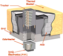 click to enlarge |
 click to enlarge |
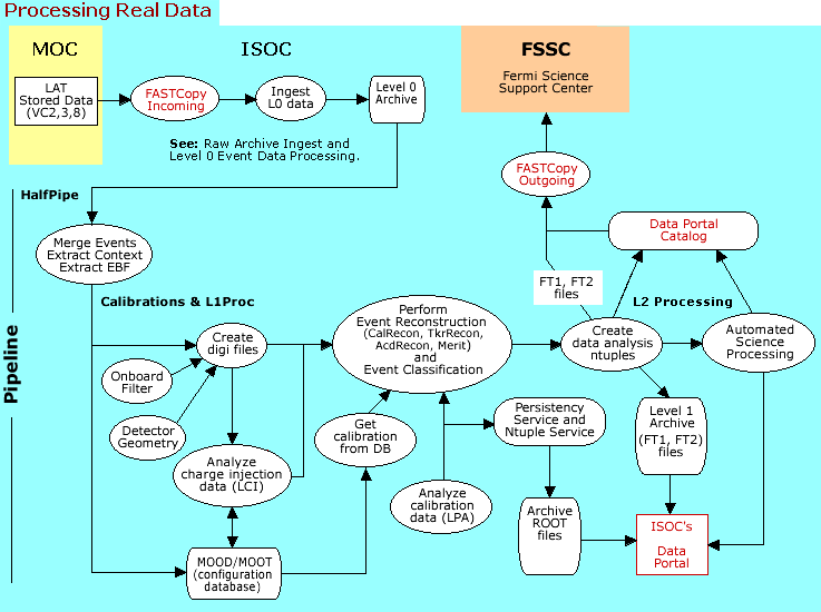
Between collection and delivery, raw data is transferred from the Mission Operations Center (MOC) to the Instrument Science Operations Center (ISOC) where it is unpacked and processed through the pipeline. The FT1 and FT2 files and the Automated Science Products (ASP) are then sent to the Fermi Science Support Center (FSSC) for widespread distribution. All data processing products are also available from the ISOC's Data Portal and Data Catalog. To ensure quality, intermediate products are monitored throughout the entire data processing chain. (See ground software's links page.) |
GLEAM Application
Photons are detected as discrete "events", consisting of the tracks (energy deposit) left by ionizing particles in different parts of the instrument. These "events" need to be classified as incident charged particles or photon-induced particle pairs. The ability to separate charged particles from gamma-ray pair events determines the level of background contaminating the sample.
Raw data received from the satellite's downlink telemetry and converted to Level 0 (L0) data is input to the Glast Event Analysis Machine (GLEAM), the reconstruction application that finds charged tracks in the Tracker (TKR) and clusters of energy deposition in the Calorimeter (CAL). Tracks are extrapolated to the Anti-Coincidence Detector (ACD) to determine whether a tile fired along the path of the track. (See Charged Particle Detection vs. Backsplash.)
Potential photons, consisting of two tracks in a "vee" (or possibly a single track, for some high energy photons), are written to an output file where they are available for further analysis.
Note: At this stage, cuts can be made to reject background events.
 Click to enlarge Click to enlarge |
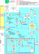
GLEAM is the top-level GlastRelease package, and its basic function is to take the "raw", Level 0 event data delivered to it in LAT Data Format (LDF) and convert it to Level 1 (L1) data ready for analysis using Science Tools software. In the diagram at left, note that Level 0 event data in LAT Data Format is read into the Gleam application by the ldfReader package (upper right). |
Notes:
- An ldf wrapper is applied to ebf data for transmission purposes. (See Level 0 Event Data Processing).
- For more information on the LAT Data Format, see Flight Software's GLAST LAT Data Format \n (LDF) \n parser package.
The LdfEvent package is used to define the LDF-specific TDS classes. The LdfConverter converts the Event inputs to digi outputs: AcdDigi, TkrDigi, CalDigi, and Trigger. (See Graphical Class Hierarchy.) Outputs are then stored in the Transient Data Store (TDS). (See Event.)
Observe that the LdfConverter outputs are also sent to the RootCnvSvc, which converts them to ROOT Tree formats (see package RootConvert) and stores them as digiRootData.
Note: For the purposes of this discussion, the digiRootData (detector) files produced at this time are optional outputs, and not used for the reconstruction of real data. The reconRootData files are reconstruction products (Acd, Tkr, and Cal) that are also stored as optional outputs. The Merit Ntuple is in ROOT Tree format, and is the primary output of GLEAM; hence, a brief description of ROOT is included below.
ROOT
ROOT is an I/O and analysis package that allows C++ objects to be stored inside a file. The I/O package is designed to create compact files, and also allows efficient access to the data. The tree structure of ROOT files allows a subset of the branches to be manipulated, thereby reducing the amount of I/O required. A C++ script extracts likely photon events and creates a new truncated ROOT file.
ROOT files containing data (whether from the satellite, simulation software, or some other source, e.g., beam test data) all have the same internal structure, allowing I/O and low-level analysis routines to be shared.
| Logical structure of raw detector data stored in ROOT. |
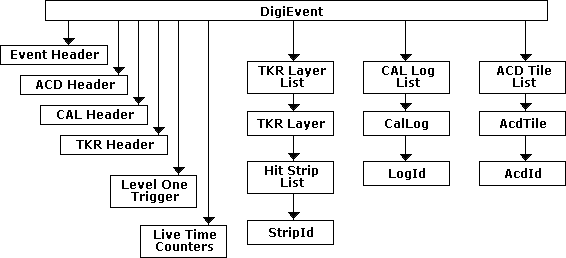 |
| Note: RootWriter converts the instrument response files (IRF) files into ROOT files. The various formats are converted into C++ objects that are then stored in a ROOT file within its tree structure; the same event structure is used for both real and simulated data. (See digiRootData.) |
After reconstructing the digitized event data, Gleam produces a reconRootData file and a summary ntuple file. (See package AnalysisNtuple and package merit; also see Standard AnalysisNtuple Variables.)
Note: GLEAM can also incorporate input from Source Generators and process Monte Carlo (MC) data using the same Reconstruction Algorithms, Transient Data Store, and Persistency and Ntuple Services that are used to process LDF data. However, this discussion focuses on the processing of real data; for the most part, generating and reconstructing MC data will be covered in a separate section.
Detector Geometry: Alignment Constants File
Note: An alignment constants file is an xml file, and is a representation of the actual alignment relationships between TKR components with respect to their ideal (i.e., perfectly aligned) relationships. These files also account for relationship discrepancies such as:
- between TKR towers.
- edge hits.
- nearly horizontal tracks.
- etc.
Elements subject to alignment:
Tower:Can be displaced with
respect to the:
- Trays
- Face
- Ladders
- Wafers
–
–
–
–Tower
Tray
Face
Ladder
Example – Alignment Constants File (for simulation):
Tower 3 Tray 1 Face 1 Face 2 Tower 4 Face 0 Ladder 1 Wafer 2 Wafer 1 Notes:
- If no constants are given, zeros are assumed.
- At each level:
- Alignment constants at that level, if any, are read in.
- Constants are merged with those from the level above
(including nulls for any not specified).- The merged constants are passed down to the next level; an array containing one entry for each wafer in the detector – 9216 in all for the flight instrument. Treatment is general; two towers is a special case.
For a much more detailed introduction
to the LAT Detector's Geometry, see:
Also see:
Basics of: Event Selection,TkrRecon, and the Calorimeter
Event Selection
Background rejection performs the function of particle identification, determining whether the incoming particle was a photon.With the high charged-particle flux in space, shower fluctuations in background interactions can mimic photon showers in non-negligible numbers. Cuts are applied to the events to suppress the background.
First, all events are reconstructed, but only events in which none of the ACD tiles fired are considered. The cut eliminates 90% of triggered events. Most of the rejected events consist of charged particles, but a few legitimate photons are also rejected if, for example, one of the particles in the shower exits the detector through the sides or top, and fires an ACD tile.
Note: This cut could be applied before any reconstruction, but reconstructing all events is useful in comparing the data with simulations.
Next, the reconstructed tracks are tested for track quality, formed from a combination of goodness-of-fit, length of track, and number of gaps on the track. Also, an energy-dependent cut removes events with tracks that undergo an excessive amount of scattering.
Finally, it is required that there be a downward-going vee in both views, and that both tracks in the vee extrapolate to the calorimeter. (This will introduce some inefficiency for high-energy photons, and for highly asymmetric electron-positron pairs. Vees with opening angles that are too large, >60o, are rejected. Such vees generally come from photons with energies below the range of interest.)
TKR Tower
A tracker tower consists of strips of silicon detectors arranged in pairs, with each element of the pair providing a separate measurement in one direction (X or Y) perpendicular to the tower axis. Reconstruction is initially done in separate Z-X and Z-Y projections. Projections are associated with each other whenever possible by matching tracks with respect to length and starting positions.
Multiple Coulomb Scattering (MS). In the absence of interactions, particle trajectories would be straight lines. However, the converter foils needed to produce the interactions (as well as the rest of the material in the detector), cause the particle to under go multiple Coulomb scattering (MS) as they traverse the tracker, complicating both pattern recognition (i.e., finding the particles) and track fitting (determining the particle trajectories), particularly for low-energy electrons and positrons. Pattern recognition must therefore be sensitive to particles whose trajectories depart significantly from straight lines.
The presence of multiple scattering also has implications for the fitting procedure. Without MS, deviations from a straight line are due solely to measurement errors, which occur independently at each measurement plane and are distributed about the true straight track. In the presence of MS, there are real random deviations from a straight line,and these deviations are correlated from one plane to the next. For example, if an individual particle scatters to the right at one plane, it is more likely to end up to the right of the original undeviated path than to the left.
Covariance Matrix. These correlations can be quantified in a covariance matrix of the measurements, which is calculated from the momentum of the particle and the amount of scattering material between the layers. The dimension of this matrix is the number of measurements. Solving for the track parameters in terms of the measurements involves inverting this matrix. If there is no MS, the matrix is diagonal, and the inversion is trivial; MS introduces off-diagonal elements, which complicates the inversion.
Kalman Filter (KF). The Kalman Filter technique can be useful in both stages of particle reconstruction. First, the initial position, direction, and energy of the particle is estimated. The energy of the particle is based on the response of the calorimeter, and the starting point and direction are derived by looking for three successive hits that line up within some limits.
From this starting point, the track is extrapolated in a straight line to the next layer. Using the estimate of the energy and the amount of material traversed, a decision is made whether the hit in the next layer is within a distance from the extrapolated track allowed by the expected multiple scattering and the uncertainty of the initial estimate. If so, the hit is added to the track, and the position and direction of the track at this plane are modified, incorporating the information from the newly added hit.
The modified track is now extrapolated to the next plane, and the process continues until there are no more planes with hits. All the correlations between layers have been properly taken into account but, at each step, only MS between two successive planes need be considered, and the covariance matrix required is that of the parameters.
The track parameters at the last hit have now been calculated using the information from all the preceding hits. To get the best estimate of the initial direction of the photon, however, it is necessary to know the parameters at the first hit, close to the point where the photon converts to an electron-positron pair.
Smoothing. At this point, smoothing is applied, i.e., the KF is "run backwards" from the last plane to the first, using the appropriate matrices. After smoothing, the track parameters, and their errors have been calculated at each of the measurement planes; in particular, the first plane.
Calorimeter
A high-energy photon traversing material loses its energy by an initial pair-production process
(λ → e+e-) followed by subsequent bremsstrahlung (e → λ) and pair production, resulting in an electromagnetic cascade, or shower. The scale length for this shower is the radiation length, the mean distance over which a high-energy electron loses all but 1/e of its initial energy.
The calorimeter provides information about the total energy of the shower, as well as the position and direction , and shape of the shower; or of the penetrating nucleus or muon. It consists of eight layers of ten CsI(TI) crystals ("logs") in a hodoscopic arrangement, i.e., alternatively oriented in X and Y directions, to provide an image of the electromagnetic shower. It is designed to measure photon energies from 20 MeV to 300 GeV and beyond.
To comfortably contain photons with energies in the 100-GeV range requires a calorimeter at least twenty radiation lengths thick. However, weight constraints forced limiting Fermi's calorimeter to only ten radiation lengths in thickness; thus, it cannot provide good shower containment for high-energy photons.
The mean fraction of the shower contained at 300 GeV is about 30% for photons at normal incidence, at which the energy observed is very different from the incident energy; the shower development fluctuations become larger, and the resolution quickly decreases.
Correcting for Shower Leakage: Method 1 (Shower-profiling) – fit a mean shower profile to observed longitudinal profile. The profile-fitting method proves to be an efficient way to correct for shower leakage, especially at low-incidence angles when the shower maximum is not contained. After the correction is applied, the resolution (as determined from a simulation) is 18% for on-axis TeV photons – an improvement by a factor of two over the result of correcting the energy with a response function based on path length and energy alone.
Correcting for Shower Leakage: Method 2 (Leakage-correction) – use the correlation between the escaping energy and the energy deposited in the last layer of the calorimeter. The last layer carries the most important information concerning the leaking energy: the total number of particles escaping through the back should be nearly proportional to the energy deposited in the last layer.
Both correction methods significantly improve the resolution. The correlation method is more robust, since it does not rely on fitting individual showers; but its validity is limited to relatively well-contained showers, making it difficult to use at more than 70 GeV for low-incidence-angle events.
Three methods are used to measure the energy deposit in the calorimeter:
- Parametric Correction (can be used for any track).
- Use the tracks to characterize the shower by:
- Position, angle
- Radiation lengths traversed
- Proximity to gaps
- Correct "raw" energy.
- Use the tracks to characterize the shower by:
- "Likelihood" (limited energy and angular range).
- Uses the relation between energy deposit in the last layer and in the rest of the shower.
Note: Below ~50 GeV, last-layer energy is proportional to the leaked energy.
- Profile Fitting (limited angular range).
- Fit layer-by-layer deposit to shower shape.
Note: Best if shower peak is contained in the calorimeter.
Choose the best answer (based on the expected error for each of the three methods). See CalRecon.
HalfPipe
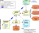
| The real, Level 0 data is received from the MOC by FASTCopy Incoming and is ingested, archived, and sent to the HalfPipe application in the processing Pipeline. | |
 click to enlarge |
See: |
Also see:
- Tips: LAT Data Processing Monitor
(FASTCopy Incoming, FASTCopy Outgoing, Monitoring Data Production, etc.)
- Monitoring Pipeline II
(For specific items to check when monitoring the Pipeline, see On a Per Run Basis.)
Note: Input to L1Proc must be one of the currently supported types:
- CCSDSFILE (for LSF "LDFFILE" for raw ldf)
- LDFFITS (for FITSified ldf)
- EBFFILE (for raw ebf)
- EBFFITS (for "slightly FITSified" ebf)
- NONE (for no real input)
See: LdfConverter - jobOptions.
Also see: LdfConverter --> File Members
L1 Processing
|
Note: You may wish to refer to the Processing Real Data diagram throughout this section. |
Create Digis
L1 Processing begins with event data output from the HalfPipe (i.e., event data in EBF format). The ldfReader presents the event data to the LdfConverter, which then writes the Acd, Tkr, and Cal digis to the event TDS.
See:
-
ldfReader – Receives the event data from the HalfPipe, parses the input, and presents it to the LdfConverter.
- LdfEvent – Defines the LDF-specific TDS classes.
- LdfConverter – LDF Online library's EventSummary marker routine determines whether or not the retrieved event is a data event. It then stores the event digis (Acd, Tkr, and Cal) in the Transient Data Store (TDS).
Also see:
MOOD/MOOT (Configuration Database)
Note that output from the HalfPipe is also input to the MOOD/MOOT configuration database. This HalfPipe output is a code that enables MOOT to retrieve all configuration-related files active at the time of the event from the MOOD database.
See:
Also See:
Get Calibration from Database and Analyze Charge Injection (LCI)
and Calibration Data (LPA)
See:
Perform Event Reconstruction and Event Classification
Event Reconstruction in a "Nutshell"
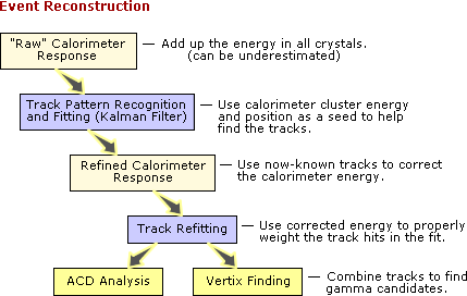
Event reconstruction is a series of sequenced operations, each implemented by one or more algorithms, and using Transient Data Store (TDS) for communication.
First, perform:
|
 |
See:
- Followed by a full CalRecon to find clusters in order to estimate energies and directions.
- Track refitting is then performed, using the corrected energy to weight the track hits in the fit.
Finally,
- AcdRecon is performed to associate tracks with hit tiles to reject events in which a tile fired in the vicinity of a track extrapolation. (See Charge Particle vs. Back Splash.)
ACD Analysis. The ACD has been measured to be ~99.97%efficient for minimum-ionizing particles; so the most interesting thing about the ACD is where it isn't, meaning that, because of gaps in the ACD coverage, charged tracks may fail to produce a signal in any tile. The ACD Analysis identifies these gaps to remove sources of background.
See: ACD Analysis.
and
- Vertex finding is performed to combine tracks in order to find gamma candidates.
(See TkrRecon --> Major Algorithms, Access to the "interesting" quantities,
and Services.)
Perform Event Classification
See Introduction to the Standard Analysis of LAT Data:
- Event Classes and Instrument Response Functions (IRFs)
- LAT Data Products --> Photon Classification
Also see:
- package GlastClassify --> Related Pages --> merittuple CTB Variables
Create Data Analysis Ntuples
The merit package implements meritAlg, which is the algorithm that:
- Copies variables from AnaTup to the output MeritTuple
- Does a point spread function (PSF)
- Does an effective area (Aeff) analysis
See:
Also see:
| Owned by: |
| Last updated by: Chuck Patterson 07/16/2010 |