Comparison of Surveyor and RIPE
Authors:
Les Cottrell
and Warren Matthews.
Created: February 23, 2000; last updated on
March 14, 2000
Introduction
Both of these tools make end-to-end active performance measurements of the Internet.
Both the
Surveyor
and RIPE
monitoring projects rely on a dedicated
PC running Unix to be placed at each monitoring site. Each PC in turn relies
on a
Global Positioning System (GPS) device to obtain accurate time
and to synchronize time
between each of the monitors. The monitors send packets at Poisson
randomized time intervals to each other and use these packets to gather
one way end-to-end delay and loss measurements. They also make concurrent
traceroutes which provides route history information. The community for
Surveyor is Internet 2,
though there are monitors at non Internet 2 sites,
and in particular at 3 Higher Energy Physics (HEP) sites
CERN, FNAL
and
SLAC that are also
PingER monitor
sites. The community for RIPE is European
Internet Service Providers (ISPs), though again there are
RIPE machines at CERN and SLAC.
More general
information comparing Surveyor and RIPE and other active measurement projects
can be found in
Comparison of some Internet
Active End-to-end Performance
Measurement projects.
Comparing Surveyor with RIPE
 We looked at 2 sets of data measured from the SLAC Surveyor and RIPE
machines. In the first set (henceforth referred to as the Jan-15 set)
we took the data from 00:00 15 January
2000 thru 23:59 January 22nd UTC. There were 197,565 Surveyor samples
and 17,168 RIPE samples in the Jan-15 data set.
In the second set (henceforth referred to as Jan-4) we took the data
from 00:00:00 January 4th, 2000 through 14:49:38 on the same day.
There were 41462 Surveyor samples and 2160 RIPE samples in this
Jan-4 data set. Both Surveyor and RIPE delay measurements were recorded
with 10 usec digit granularity. The Surveyor timestamps were recorded with
100 usec. granularity and the RIPE timestamps with 1 usec. digit graunularity.
Jan-15 Data Set
Since the autocorrelation functions of pings measured as closely apart
as 1 second (see
High statistics ping results) indicate very weak correlations,
rather than look for correlations between individual Surveyor and RIPE
probes we look at the data in aggregation.
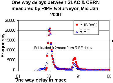
Therefore, for the Jan-15 set, we binned the RIPE & Surveyor data
into 0.1 millisecond bins and plotted the
one-way delay time distributions that are shown to the right.
In the figure RIPE data has been normalized so the peak height of the 1st peak
around 86 msec. has the same height as the equivalent peak in the
Surveyor distribution. Also
0.2 msec. have been subtracted from the delays for the RIPE data to improve
the agreement, this is discussed in further detail below.
It can be seen that there is reasonably good agreement. Looking in more detail
it is noteworthy that the second peak at around 95 msec. has more counts for the
Surveyor data. Also there is more RIPE data at lower delays in the region
below the 1st peak. These difference are due to the 2 experiments
not both being up during the entire
interval and therefore not measuring exactly the same behavior. In particular
the SLAC Surveyor machine didn't take data during the period when the SLAC
RIPE machine was reporting one-way delay less than 90ms.
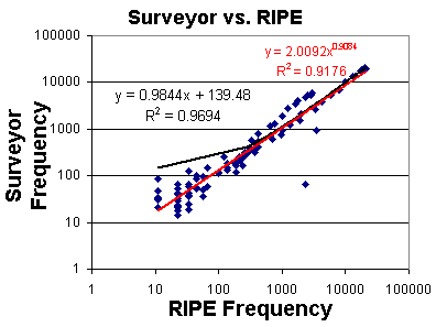 We then scatter plotted the two distributions against one another, i.e. each
point on the scatter plot is for a given delay and has an x-value equal to the
normalized RIP frequency for that delay, and the y-value is the
Surveyor frequency for the same delay. The plot of this data can be
seen to the left. The black line is a linear least squares fit
of y to a straight line in x, and the red line is for a linear least
squares it to a power series.
It can be seen that there is a strong correlation between the points with
R2 > 0.9 (i.e. the proportion of variation in the
Surveyor distribution attributable to the RIPE distribution is over 90%,
see "The New Statistical Analysis of Data", by T. W. Anderson and
Jeremy D. Finn, published by Springer, 1996).
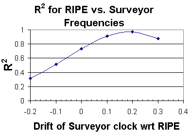 Then we plotted the R2 of the scatter plot data
as a function of the "correction" (drift) made to the
Surveyor delay. The plot of this is seen to the right.
It can be seen that the best correlation
(highest value of R2)
is obtained when the Surveyor delay times are increased by 0.2 msec.
Some of this difference maybe attributable to the differences in packet sizes of
the probes used. Surveyor uses 40 Byte packets whereas RIPE uses 100 Byte packets.
For larger packets delay will be higher.
Henk Uijterwaal of RIPE-NCC reports: "I've measured this effect for the path
Advanced-RIPE and back last April 1999,
and found differences of 0.4..0.6 ms (depending on the time of day and
thus network load). One can calculate the effective throughput from
these numbers. Back in
April, I ended up with something in the 80 to 120 kb/s range, which is
consistent with what one sees when transferring large files between the
two sites. Of course, the numbers may be different for the
SLAC-CERN connection, but
delays for the RIPE box should be a little higher than for Surveyor."
Jan-4 Data set
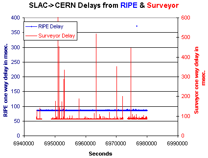 To avoid the different coverages of the RIPE & Surveyor data we chose the
second data set (Jan-4) so the coverages would match more closely. The figure to the left
shows the RIPE and Surveyor one-way delay time series for the Jan-4 data set. In
order to help the two series stand apart they are plotted against different
y axes. The x axis is the Unix epochal seconds since 00:00:00 Jan 1st 1970.
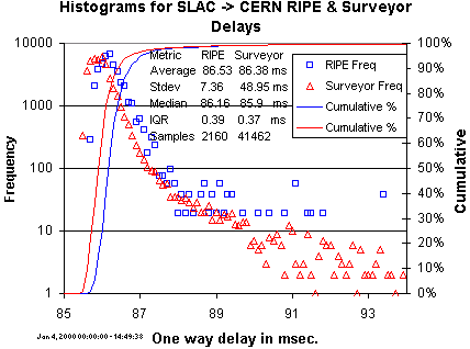 The frequency histograms for the RIPE and Surveyor Jan-4 data set is shown
to the right together with relevant values for the median, average, standard
deviation (Stdev), inter quartile range (IQR) and
the number of samples. The Frequency is plotted as a log scale to illustrate
the
heavy tailed behavior. The RIPE frequencies have been normalized to have the
same number of samples as
Surveyor's, so the plots can be overlaid.
It can be seen that the outliers in the Surveyor
data result in a much higher standard deviation. The peaks have similar widths
as measured by the IQR, but the medians (and averages) for the RIPE and
Surveyor measurement differ by 0.1
to 0.26 msec.
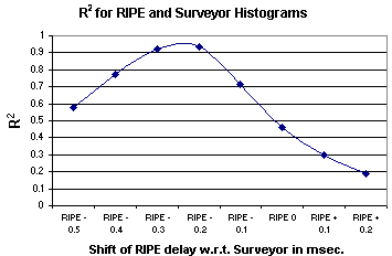 To pin point the differences of the median delays between the RIPE and
Surveyor measurements, we adjusted the RIPE delays in the range of -0.5 msec. to
+0.2 msec. in steps of 0.1 msec. For each of these adjusted delays we compared
the frequency histogram points for each value of the delay by calculating
the square of the correlation coefficient (R2) and plotting
it as a function of the adjustment made to the RIPE delays. It can be seen that
the in the chart to the left that the optimum fit
(largest value of R2) is when between
0.2 and 0.3 msec are subtracted from the RIPE delays.
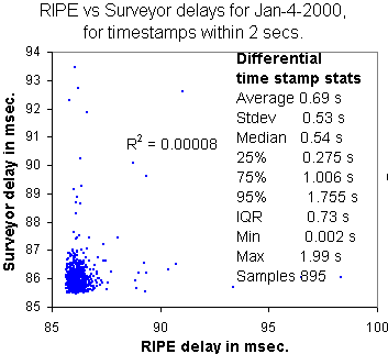 To compare the individual measurements made by RIPE and Surveyor,
for each of the ~2160 RIPE measurements we took the Surveyor
measurement immediately preceding the RIPE measurement.
Then we took the difference in the timestamps, i.e.
dTi = TSi - TRi for
each pair (with index i),
where TSi is the timestamp of the i-th
Surveyor delay measurent and
TRi is the same for the RIPE delay measurement.
Then we sorted by differential dT, and kept those pairs that had a
dT of < 2 secs. Then we scatter plotted
these points and caluculated the R2. We also looked at the dT
distribution. The results are shown to the right. This may illustrate
that for this data, even for meaurements close togther in time
(< 2 seconds apart and a median separation of 0.545 seconds),
there is little correlation between the points.
This is even though there are points that have long delays,
the problem is that the
long delays in one measurement are not reflected in the other measurement.
Presumably this means that the effect that
caused the long delay in one measurement has change its effect by the
time (< 2 secs later) the other measurement is made.
To obtain stronger correlation one probably
needs more data with a persistent structure in the data (for
example such as would be caused by a routing change or congestion). An example of
data with more structure can be seen in the results reported in
Comparison of Surveyor and PingER.
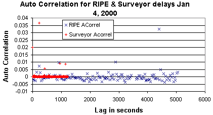 To see whether there was any point is trying to correlate individual delay measurements
made at similar time stamps, we plotted the auto correlation values for the RIPE
and Surveyor data. They are seen to the right. It can be seen that at these time scales
and for the Jan-4 data set the auto-correlation is small even for small values
of the Lag (the minimal lag or average separation between adjacent samples
for RIPE is about 40 seconds, and for Surveyor it is about 1 second) the
auto correlation has a very small value.
Conclusions
To effectively compare the methods it is important to ensure that
the measurements cover the same time periods.
The RIPE and Surveyor delay distributions strongly correlate (i.e. over 90%
of the Surveyor variation in the delay distribution in Surveyor
is attributable to
the delay distribution for RIPE). The widths of the distributions and the
percentiles are also similar. The offset of about 0.2-0.3 msec.
in the modes of the distributions can be explained by the difference
in packet sizes. The lack of any long term (i.e. behavior persistent over time
periods of 0.5 seconds or more)
structure in the data results in there being little correlation between
the Surveyor and RIPE data points. The lack of
a strong auto correlation value for the delays measured by RIPE
and Surveyor for these data sets is also probably due to the lack of noticeable
structure in the data.
[ Feedback ]
 We then scatter plotted the two distributions against one another, i.e. each
point on the scatter plot is for a given delay and has an x-value equal to the
normalized RIP frequency for that delay, and the y-value is the
Surveyor frequency for the same delay. The plot of this data can be
seen to the left. The black line is a linear least squares fit
of y to a straight line in x, and the red line is for a linear least
squares it to a power series.
 We looked at 2 sets of data measured from the SLAC Surveyor and RIPE
machines. In the first set (henceforth referred to as the Jan-15 set)
we took the data from 00:00 15 January
2000 thru 23:59 January 22nd UTC. There were 197,565 Surveyor samples
and 17,168 RIPE samples in the Jan-15 data set.
In the second set (henceforth referred to as Jan-4) we took the data
from 00:00:00 January 4th, 2000 through 14:49:38 on the same day.
There were 41462 Surveyor samples and 2160 RIPE samples in this
Jan-4 data set. Both Surveyor and RIPE delay measurements were recorded
with 10 usec digit granularity. The Surveyor timestamps were recorded with
100 usec. granularity and the RIPE timestamps with 1 usec. digit graunularity.
 Then we plotted the R2 of the scatter plot data
as a function of the "correction" (drift) made to the
Surveyor delay. The plot of this is seen to the right.
 To avoid the different coverages of the RIPE & Surveyor data we chose the
second data set (Jan-4) so the coverages would match more closely. The figure to the left
shows the RIPE and Surveyor one-way delay time series for the Jan-4 data set. In
order to help the two series stand apart they are plotted against different
y axes. The x axis is the Unix epochal seconds since 00:00:00 Jan 1st 1970.
 The frequency histograms for the RIPE and Surveyor Jan-4 data set is shown
to the right together with relevant values for the median, average, standard
deviation (Stdev), inter quartile range (IQR) and
the number of samples. The Frequency is plotted as a log scale to illustrate
the
heavy tailed behavior. The RIPE frequencies have been normalized to have the
same number of samples as
Surveyor's, so the plots can be overlaid.
It can be seen that the outliers in the Surveyor
data result in a much higher standard deviation. The peaks have similar widths
as measured by the IQR, but the medians (and averages) for the RIPE and
Surveyor measurement differ by 0.1
to 0.26 msec.
 To pin point the differences of the median delays between the RIPE and
Surveyor measurements, we adjusted the RIPE delays in the range of -0.5 msec. to
+0.2 msec. in steps of 0.1 msec. For each of these adjusted delays we compared
the frequency histogram points for each value of the delay by calculating
the square of the correlation coefficient (R2) and plotting
it as a function of the adjustment made to the RIPE delays. It can be seen that
the in the chart to the left that the optimum fit
(largest value of R2) is when between
0.2 and 0.3 msec are subtracted from the RIPE delays.
 To compare the individual measurements made by RIPE and Surveyor,
for each of the ~2160 RIPE measurements we took the Surveyor
measurement immediately preceding the RIPE measurement.
Then we took the difference in the timestamps, i.e.
dTi = TSi - TRi for
each pair (with index i),
where TSi is the timestamp of the i-th
Surveyor delay measurent and
TRi is the same for the RIPE delay measurement.
Then we sorted by differential dT, and kept those pairs that had a
dT of < 2 secs. Then we scatter plotted
these points and caluculated the R2. We also looked at the dT
distribution. The results are shown to the right. This may illustrate
that for this data, even for meaurements close togther in time
(< 2 seconds apart and a median separation of 0.545 seconds),
there is little correlation between the points.
This is even though there are points that have long delays,
the problem is that the
long delays in one measurement are not reflected in the other measurement.
Presumably this means that the effect that
caused the long delay in one measurement has change its effect by the
time (< 2 secs later) the other measurement is made.
To obtain stronger correlation one probably
needs more data with a persistent structure in the data (for
example such as would be caused by a routing change or congestion). An example of
data with more structure can be seen in the results reported in
 To see whether there was any point is trying to correlate individual delay measurements
made at similar time stamps, we plotted the auto correlation values for the RIPE
and Surveyor data. They are seen to the right. It can be seen that at these time scales
and for the Jan-4 data set the auto-correlation is small even for small values
of the Lag (the minimal lag or average separation between adjacent samples
for RIPE is about 40 seconds, and for Surveyor it is about 1 second) the
auto correlation has a very small value.