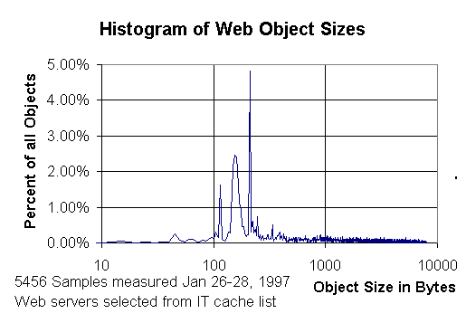
Figure 1 shows the frequency histogram of the sizes of web objects in the IT cache list.
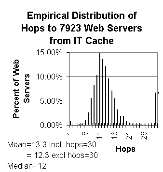
Figure 2 shows a typical hop count distribution. About 10% of the traceroute hop measurements returned hop counts of 30, the default maximum hop count.
Les Cottrell and John Halperin Stanford Linear Accelerator Center (SLAC)
We investigate the correlation of the network response times to those of Web retrieval. The network response times to Web servers is estimated using the well known ping utility response times. The Web retrievals use the standard HyperText Transport Protocol (HTTP [HTTP]) GET (henceforth referred to as a GET). Such information is needed to identify how Web responsiveness may be affected by the network.
The measurement program applied successive filters to restrict the URLs used, the measurements made and the samples recorded for further analysis. An example of how the filters progressively restricted the input passed to the next filter is seen in Table 1 below. The information is provided here to help clarify the measurement process, and to give an idea of the frequency of some of the failures seen on the Internet.
| Stage | Filter | Number of Inputs to Filter | Number Rejected by Filter | % Rejected |
|---|---|---|---|---|
| Check Cache URLs | URL contains "invalid characters" | 131069 | 2772 | 2.11% |
| Check Cache URLs | URL scheme is not "http" protocol | 128297 | 1505 | 1.17% |
| Check Cache URLs | Path name contains "cgi" | 126792 | 691 | 0.54% |
| Check Cache URLs | Duplicate host, i.e. host already successfully measured | 126101 | 110927 | 87.97% |
| Xchkaccess (GET) | Host Name Invalid or Unknown | 15174 | 630 | 4.15% |
| Xchkaccess (GET) | TCP Connection Rejected | 14544 | 207 | 1.42% |
| Xchkaccess (GET) | Time Out (20 seconds) | 14337 | 1447 | 10.09% |
| Xchkaccess (GET) | Error in read response from server | 12890 | 2 | 0.02% |
| GET Response Size | Response has 0 bytes | 12888 | 101 | 0.78% |
| GET Response Size | Response size outside threshold (> 8KB) | 12787 | 3618 | 28.29% |
| Ping | 100% packet loss | 9169 | 393 | 4.29% |
| Ping | Pathological Pings (e.g. duplicate responses) | 8776 | 17 | 0.19% |
| Httpq | httpq fails | 8759 | 16 | 0.18% |
| Successfully Measured Samples | Analysis Program | 8744 |
For each successful measurement, we recorded one record with the: timestamp, hostname, port, path name, GET response size, the server type and the HTTP status code, and relevant information from the cache list (e.g. the cache list's measure of the GET response size, and transfer time). The record also contains: for each set of 10 GETs, the median, the 25 percentile, the 75 percentile and inter-quartile range and the first GET responses; for each set of 10 pings, the average, minimum and maximum* responses, plus the percentage of ping packets lost. The granularity of the clock as reported was 1 millisecond for ping and for xchkaccess.
For the URLs successfully retrieved using the IT cache list, about 45% had the suffix .gif, ~35% had .htm, .html or .shtml, ~7% had .jpg, ~10% had no suffix, and the other main suffixes observed were .asp, .class, .js, .exe, .txt and .xbm. About 70% of the GET responses had HTTP status codes of 200 (OK, the request was fulfilled), about 18% had code 404 (server could not find given resource), about 10% had code 302 (suggestion for the client to try another location), and about 1% had code 401 (client is not authorized to access data). The remaining 1% was mainly composed of codes 301, 403, and 400. The top 5 identified WWW servers were from Apache (41%), Netscape (18%), NCSA (15%), WebSite (4%) and CERN (3%). For a survey on Web server software usage see The Netcraft Web Server Survey.
A typical GET response size distribution is seen in Figure 1. The sharp peaks in the GET response distribution are associated with specific response such as the server reporting that it is unable to find a requested object. For example the peak at 207 bytes is largely composed of status code 404 responses from a particular brand of server.
Figure 1 shows the frequency histogram of the sizes of web objects
in the IT cache list.
Figure 2 shows a typical hop count distribution. About 10%
of the traceroute hop measurements returned hop counts of 30, the
default maximum hop count.
The distributions of the minimum (of 10) ping responses for
different bin sizes (10ms and about 120ms) are seen in Figures 3 and 4.
The ping response is
plotted on a logarithmic scale to enable one to
see more clearly the distribution for the short responses. A definite
bimodal behavior is seen in the first plot (narrower bins)
with peaks at roughly 50 msec. and 100 msec.
Note that the ping payloads for the distribution in Figures 3 and 4
follow that shown in Figure 1.
A similar distribution is obtained
for pings of a fixed payload of 1000 bytes, so the bimodality
is not believed to be due to the peakiness of the
Web object size distribution shown in Figure 1.
For the wider
bins, the distribution roughly follows a power law
(R2=0.97)
whose equation is shown in the figure.
A large difference
in the hop and ping distributions can be noticed.
Figure 3 shows a frequency histogram of the minimum ping
response time of a sample of 10076 web servers. The bin width
is 10 msec.
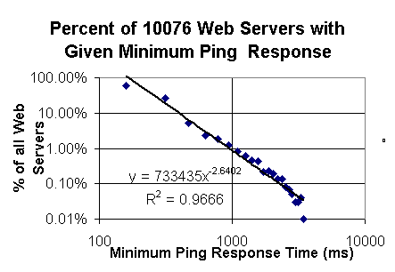
Figure 4 shows the frequency histogram of the minimum response ping
response time of the same sample of 10076 hosts seen in Figure 3,
but with a bin width of 120 msec. the curve is a power law fit to the
data with the parameters shown. the R2 [AF] of the fit is
also shown.
The distribution of the median (of 10) GET responses, for 6578 Web servers selected from the IT cache list, for 2 different bin sizes is seen in Figures 5 and 6. There is some evidence of bimodaility and again the distribution to the right of the peaks roughly follows a power law (R2=0.95).
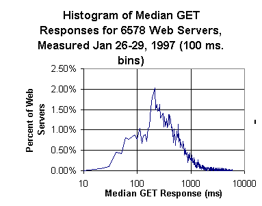
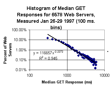
Figures 5 & 6 show the frequency hiostograms of the median
HTTP GET reponse for objects from a sample of 6578 web servers.
Figure 5 is for 10 msec. bins and figure 6 is for 100 msec. bins.
the line in figure 6 is a power law fit with the parameters
and R2 shown.
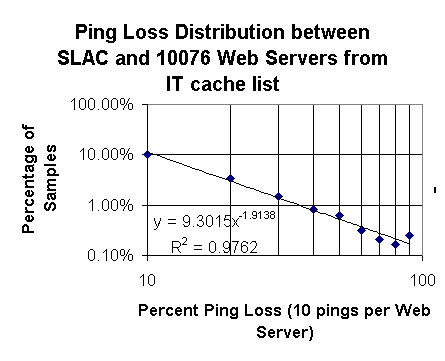
Figure 7 shows the frequency histogram of the ping losses observed
to 10076 web servers in the IT cache list. A power law fit
is also shown together with its parameters and R2.
The statistics of the GET response sizes and the response times are summarized in Table 2. The "Min.", "Avg." and "Max." refer to the minimum, average and maximum of the 10 pings or 10 GETs done for each host.
| Statistics | GET Response Size (Bytes) | Min. GET (msec.) | Min. Ping (msec.) | Avg. GET (msec.) | Avg. Ping (msec.) | Max. GET (msec.) | Max. Ping (msec.) | Median GET (msec) |
|---|---|---|---|---|---|---|---|---|
| 25 Percentile | 331, 331 | 216, 217 | 87, 87 | 288, 297 | 96, 94 | 440, 433 | 114, 106 | 254, 253 |
| 50 Percentile | 1602, 1562 | 393, 376 | 132, 127 | 554, 538 | 151, 140 | 826, 786 | 193, 174 | 461, 458 |
| 75 Percentile | 3534, 3537 | 657, 624 | 205, 177 | 1027, 936 | 237, 201 | 1897, 1716 | 318, 260 | 852, 745 |
| Average | 2230, 2246 | 568, 525 | 215, 178 | 884, 803 | 252, 207 | 1927,1788 | 322, 262 | 733, 664 |
| Standard Deviation | 3106, 2132 | 710, 664 | 359, 288 | 1107, 978 | 456, 386 | 2733, 2509 | 585, 515 | 973, 880 |
| Minimum | 11, 11 | 11, 15 | 1, 2 | 13, 16 | 3, 2 | 16, 19 | 4, 2 | 12, 15 |
| Maximum | 7991, 7999 | 16454, 12218 | 12152, 12633 | 16582, 14118 | 12152, 11085 | 20043, 19966 | 15363, 12633 | 16565, 14587 |
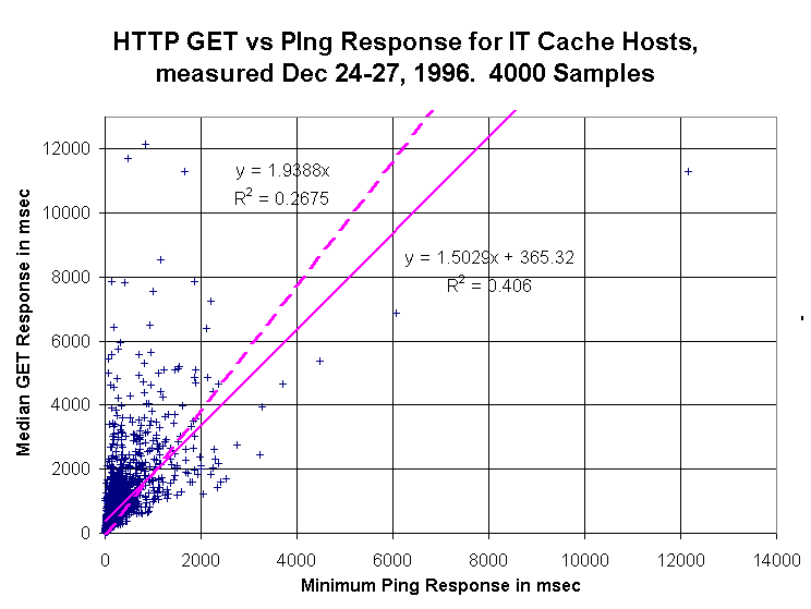
A typical scatter plot of GET versus ping response time for 4000 (the maximum plottable by Excel [MS]) successful samples is shown below in Figure 8.
The Correlation Coefficient R is defined as
[MS]:
R = COV(x,y) / (sx * sy),
where:
COV(x,y) = (1/n) * SUM((xi-xm)*(yi-ym)),
and the SUM is over the n samples (i=1..n) , also
xm = (1/n) * SUM(xi)); ym = (1/n) * SUM(yi)), and
sx2 = (1/n) * SUM((xi-xm)2); sy2 = (1/n) * SUM((yi-ym)2).
Anderson and Finn
[AF] indicate that absolute values of Rin the
range of:
0 < |R| < 0.3 indicate a "weak" correlation,
0.3 < |R| < 0.6 indicate a "moderate" correlation, and
0.6 < |R| < 1 indicate a "strong" correlation.
The square of the Correlation Coefficient (R2) defines the fraction of the total variance of y that is accounted for by its regression on x [CDM]. 1 - R2 represents the proportion of the total variability of the y values that is not accounted for by the variable x.
Table 3 shows the Correlation Coefficients for various combinations of the minimum, average and maximum ping* and the minimum, average, maximum and median GET responses for sets of 10 pings and 10 GETs for each host in a sample set of the first 4031 samples taken from the IT cache sample sets of Tables 1 and 2.
| Correlation Coefficient R | Min. GET | Avg. GET | Max. GET | Median GET |
|---|---|---|---|---|
| Min Ping | 0.609 | 0.579 | 0.36 | 0.61 |
| Avg. Ping | 0.583 | 0.558 | 0.35 | 0.587 |
| Max. Ping | 0.538 | 0.521 | 0.331 | 0.546 |
Table 3 shows that the correlation is best if we use the minimum of the 10 ping responses for each host. It might be expected that this would give better estimates of the ping response since the minimum ping response has a lower bound, whereas the maximum is unbounded and so outliers may make the average a less reliable estimator. Similar effects are seen for the GET correlations. The correlations of the minimum, average and median GET response times versus the minimum ping responses times may be said to be between "moderate" and "strong" [AF].
Further correlation improvements can be made if one ignores outlying samples with large GET response times. For example, for the set of 6000 IT cache samples described in Table 2, the Correlation Coefficients R for the minimum and median GETs versus the minimum pings increase by 16% (from 0.595 to 0.698 for the minimum GETs) and 8% (from 0.594 to 0.645 for the median GETs) if one excludes the less than 1% of the samples which have average GET response times of 6 seconds or more. A rationale for removing these samples is that they represent hosts where the GET response time is dominated by effects other than the network, such as an overloaded Web server, a slow host, or the URL invokes a CGI script etc.
| Slope | Min. GET | Avg. GET | Median GET |
|---|---|---|---|
| Min. Ping | 1.18 | 1.77 | 1.61 |
| Avg. Ping | 0.88 | 1.36 | 1.23 |
| Intercept | Min. GET | Avg. GET | Median GET |
| Min. Ping | 315ms | 502ms | 422ms |
| Avg. Ping | 345ms | 540ms | 386ms |
Typical linear regression fit slopes and intercepts are shown in Table 4 for various combinations of minimum, average and median GET responses versus minimum and average ping responses.
To evaluate whether the results are skewed by path names ending in a
slash (/), which we refer to as "index pages", which may require
the server to compose a directory listing which in
turn may take more time, we re-analyzed the data excluding samples with
such path names. These paths comprised about 25% of the paths that we
measured.
Table 5 below shows that the difference
in Correlation Coefficient if one includes or excludes "index pages" is
negligible.
| Correlation Coefficient R | Min. GET | Avg. GET | Median GET | Number of Samples |
|---|---|---|---|---|
| All samples | 0.609 | 0.579 | 0.61 | 4031 |
| All samples - Index Pages | 0.593 | 0.562 | 0.596 | 3120 |
There was a weak correlation (R ~ 0.15 - 0.19) between the minimum ping response times and the GET response sizes in bytes. There was a slightly larger but still weak correlation (R ~ 0.20 - 0.23) between the minimum or median GET response times and the GET response sizes in bytes. In one measurement run of about 1700 samples, we fixed the ping payload to 1000 bytes, instead of making the ping payload size equal to the GET response size. The Correlation Coefficient R for minimum, average and median GET response against the minimum ping response dropped by about 25% to about R=0.45 as can be seen in Table 6.
| Correlation Coefficient R | Min. GET | Avg. GET | Median GET |
|---|---|---|---|
| Min. Ping | 0.43 | 0.46 | 0.45 |
| Avg. Ping | 0.38 | 0.42 | 0.41 |
We also plotted the GET response times versus the packet loss, but could find only weak correlations (R ~ 0.18 - .24).
There was a significant difference in R between the IT and BO cache measurements. For example, for 2 sets of 6000 samples shown in Table 2 which were measured over the same time interval (December 24-28, 1996) R is as shown in Table 7. This difference is not currently understood.
| R for IT cache list hosts | Min. GET | Avg. GET | Median GET |
|---|---|---|---|
| Min. Ping | 0.595 | 0.575 | 0.594 |
| R for BO cache list hosts | Min. GET | Avg. GET | Median GET |
| Min. Ping | 0.530 | 0.511 | 0.529 |
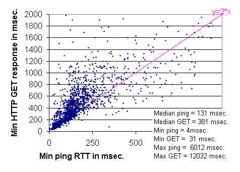
The lower boundary can also be visualized by displaying the distribution of residuals
between the measurements and the line y = 2 x (where y =
HTTP GET response time and x =
Minimum ping response time). Such a distribution is shown below. The steep in crease in
the frequency of measurements as one approaches zero residual value
(y=2x) is apparent.
The Inter Quartile Range (IQR), the residual range between where
25% and 75% of the
measurements fall, is about 220 msec, and is indicated on the plot by the
red line.
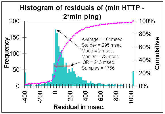
Figure 10 shows the frequency histogram of the residual of
minimum(HTTP GET response) - minimum(ping RTT response) for the
data shown in figure 9.
Other observations include:
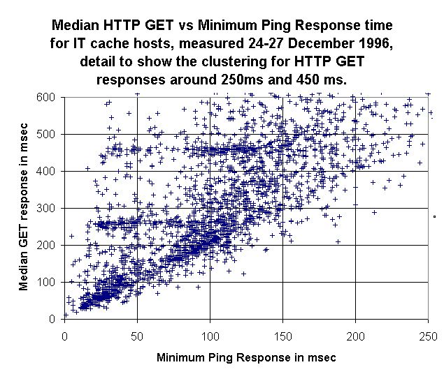
The first cluster is around median GET responses of 250-265 msec. and a further cluster at 450-465 msec. can be observed. Histogramming the frequency of median GET responses against the median GET response time (see Figure 3) shows several distinct peaks at which are separated by about 200ms.
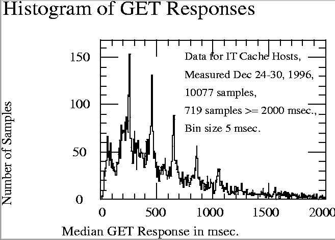
Figure 12 shows the frequency histogram of the GET reponse data in
figure 11.
Samples comprising these peaks, compared with the complete sample set, do not contain statistically significant different distributions of:
No such peaks are seen in the equivalent histogram of ping response times, though the ping responses do appear to be bimodal with a peak at about 28 msec and a larger peak at 106msec. The GET effect is reproducible across several monitoring host architectures including RS/6000 models 320H and 250 (both running AIX 3.2.5) and a Sun 4/50 running SunOS 4.1 all located at SLAC, and a Sun SuperSparc 10 running SunOS 4.1 located at the Fermi National Accelerator Laboratory (FNAL). For these different monitoring hosts, the location of the first GET response peak peak changes, for example, it is at about 320 msec. for a RS/6000 320H, about 255 msec for an RS/6000 250 and 210 msec for a Sun 4/50. However the separation of the peaks stays fairly constant at about 200msec.
The effect was an artifact of the measurement method, where the repeated GETs (up to 10) tended to synchronize with the delayed ACK timer [ST]. the solution was to delay the request for the second and consecutive GETs by a random time. The clue to this was provided by Vern Paxson.
* For later measurements we also measured the median ping response. For these measurements (about 1900 samples), the Correlation Coefficient obtained using the average ping versus the minimum, average or median GET differed from that obtained using the median ping by of the order of 1%, which was within the expected statistical fluctuations. For the bulk of the measurements and analysis we focussed on the minimum and average ping responses rather than the median ping response. This was since the summary report from the standard ping tool used by most users provides the minimum, average and maximum responses and not the median .
[AF] The New Statistical Analysis of Data, T. W. Anderson & Jeremy D. Finn, Springer Verlag, 1996
[CDM] Statistics Manual, E, L, Crow, F. A. Davis, M. W. Maxfield, Dover Publications Inc.
[CGI] The Common Gateway Interface, University of Illinois Urbana - Champaign, NCSA. http://hoohoo.ncsa.uiuc.edu/cgi/overview.html
[HTTP] HTTP - Specifications and Reports, W3C. http://www.w3.org/pub/WWW/Protocols/HTTP/specs.html
[KC] Kimberly Claffy of NLANR kindly provided access to this database, as well as an explanation and analysis of the information it contains.
[MB] Ping o' Death, Mike Bremford http://www.sophist.demon.co.uk/ping/index.html
[MS] Microsoft Excel User's Guide, version 5, Microsoft Corporation, 1994
[ST] TCP/IP Illustrated Volume 1 The ProtocolsW. Richard Stevens, Addison-Wesley Company (1994).
[ Feedback ]