Preface

Here is a conceptual overview of the technique used at SLAC to use the transient response of a pair of high Q cavities coupled to a klystron's output to achieve RF pulse compression. Technique is called SLED. In this write-up, I'll try to walk you through the pieces necessary to put together the bigger picture of the SLED technique.

This overview is deliberately not rigorous, favoring instead the relevant concepts behind the technique. A good place to look for a more rigorous treatment is in a paper called "SLED: A Method of Doubling SLAC's Energy" (1974) by Farkas, Hogg, Loew and Wilson (SLAC Pub.#1453).

Start with a very simple scheme:

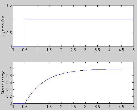
Consider a klystron coupled to a waveguide whose output is then directed to the outside world as in Figure 1:

Figure 1

RF power flows from the klystron through the waveguide and out into the surrounding medium. One can think of an RF wave of amplitude V_f travelling from left to right as shown in the figure 1. This scheme would not be very interesting for use in accelerators. It looks more like what one might want to do if one were interested in broadcasting a television signal.

Next complicate the matter a bit...

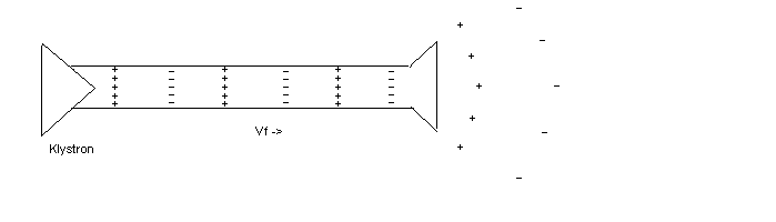
Suppose that at the end of the waveguide an iris type termination is put in place as shown here in Figure 2:

Figure 2

Since the termination shown is not a good impedence match, not all of the RF power escapes. Some of the klystron output V_f is reflected backward (shown as V_r in figure 2) towards the klystron. The RF which escapes is shown here as V_t. Normally a condition in which V_r is large would be a problem for a klystron, but let's just handle that problem later...

Now Direct the RF into some sort of RF Cavity

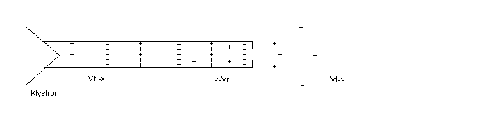
Consider now a setup as shown in Figure 3:

Figure 3

In this scheme the klyston output is directed into a resonant cavity. This picture starts to look like what one would see if considering an RF cavity for a storage ring accelerator. Here I have deliberately shown a poor impedence match to the cavity, and as a result there is a reflected wave V_r directed back towards the klystron. I have chosen a reflection coefficient R such that:

V_r = R*V_f and V_t = (1-R)*V_f

The transmitted wave V_t rattles back and forth inside the RF cavity. After klystron turn-on the amplitude of the fields inside the cavity build with time, and the energy stored in the cavity (U_c) grows. In time, the system will come to equilibrium when the available klystron power directed into to cavity (V_t) balances the energy loss rate in the cavity walls together with the power which leaks back out the coupling iris. The V_r shown in figure 3 is again the RF from the klystron reflected by the coupling iris. Not shown in figure 3 are the fields emitted from the iris due to the energy stored in the cavity.

For a moment here let's pretend the klystron is gone.

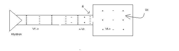
Consider a similar configuration and remove the klystron while somehow still having RF energy stored in the RF cavity. Some of the cavity's energy (U_c) leaks out the iris as shown in Figure 4:

Figure 4

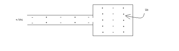
The RF wave propagating away from the RF cavity has an amplitude which I'll call V_rc. The power of this wave (goes as V_rc² ) is directly proportional to the energy stored in the cavity.

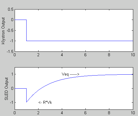
Refering back to an arrangement such as shown in figure 3 above, we would then expect the cavity stored energy to grow as shown on the bottom of plot 1 below:

Plot 1: Time evolution of SLED cavity stored energy from Figure 3.

In the literature, there is a parameter called "beta" which is a parameter of the cavity and coupling iris geometry. "Beta" is defined in such a way to represent the ratio of power emitted from the iris (due to RF in the cavity) to power lost in the cavity walls. "Beta" is often refered to as a "cavity coupling coefficient" or a "transformer ratio". A large value for beta means energy escapes quickly through the iris. Beta greater than one is called "overcoupled". For SLED the beta value worked out to be about 5.

Remember from figure 3 that after klystron turns on the system comes to equilibrium once the fields in the cavity reach a point that the wall losses together with the leakage out the iris together "consume" all of the RF (V_t) provided by the klystron. It should seem reasonably intuitive that the iris geometry (beta) and the cavity Q together determine the fill/decay time constant of the cavity. SLED parameters work out such that the SLED cavity fill/decay time constant (T_c) is about 1.8 microseconds.

Introducing the "3dB Hybrid Coupler":

There exists a microwave component called a "3dB Hybrid Coupler". Like many microwave inventions, it has some interestingly useful properties. The 3dB coupler is a four port device as shown in figure 5 below. There are two important "rules of thumb" for our purpose associated with the 3dB Coupler:

Figure 5

Rule #1:

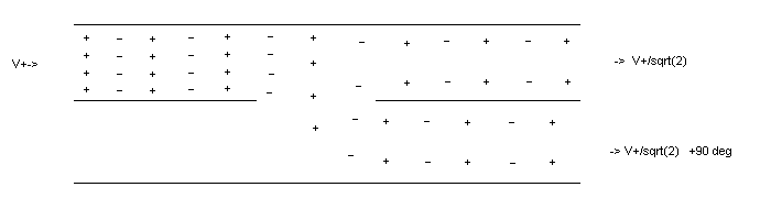
RF power directed at any one port of the coupler is directed equally (in magnetude) between the two ports opposite. Always keep in mind that power goes as the square of the field/voltage, so there are some sqrt(2) terms which have to get kicked around.

Rule #2:

The RF emitted by two ports from a wave directed at the coupler exhibit a 90 degree difference in phase.

Let's put it to use:

Let's build something similar to what we had before, but this time use the 3dB coupler as well. We can apply the two "Rules of Thumb" above to see what happens. Consider a setup as shown in Figure 6 below. Again we have mismatched irises (much as in Figure 2) but this time we use the 3dB coupler to form a pair:

Figure 6

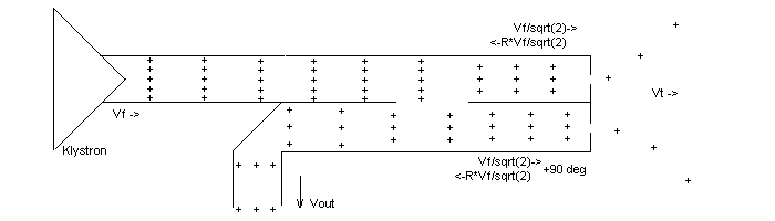
Some of the RF escapes to the outside due to leakage out the irises. The RF which leaks out the two irises have equal amplitude (3dB coupler rule #1), and the RF leaking out the lower iris is advanced by 90 deg with respect to the top iris (3dB coupler rule #2).

If the klystron forward output is V_f, then the forward (toward the irises) RF after the coupler is V_f/sqrt(2) in both the upper and lower waveguide between the coupler and the irises. The RF reflected off the irises is then R*V_f/sqrt(2) in both the top and bottom waveguide; offset by 90 degrees.

Next look at what happens to the iris-reflected RF as it goes back through the 3dB coupler. Half the reflection from the top iris goes back towards the klystron with no phase shift. Half the reflection from the bottom iris is also reflected towards the klystron, with an additional 90 degree shift; or a total shift of 180 degrees. Since the two iris reflected waves have equal amplitude but a cumulative 180 degree phase shift between them, their sum cancels. In this scheme no power is reflected back towards the klystron.

Looking at what goes to the bottom left (output) port, the two iris reflected waves combine, and each has experienced a 90 degree shift (one before reflection, one after) so they have the same phase. Adding up the numbers gives:

V_out = R*V_f

So far we have not accomplished much, other than letting some of the RF escape out the irises at the cost of reducing available output (reflection coeffiecient R is bound between 0 and 1). Not to worry, things get rather interesting pretty soon here...

Here's the Final Plumbing Configuration:

Figure 7

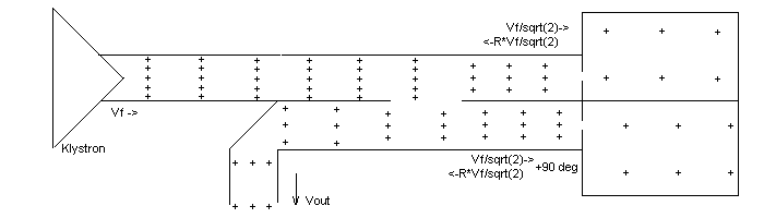
In this configuration the RF which appears at the lower left port is the superposition of two waves. The first wave (call it the "prompt wave") is just that which appeared as V_out in Figure 6, namely the klystron power reflected directly off the irises. An additional wave appears (call it the cavity radiated wave; V_rc as in Figure 4) which exhibits a time structure which evolves as the cavity stored energy builds.

Careful application of the 3dB coupler rules tell us that the two cavities radiated waves cancel at the klyston port, and add in phase together at the output port.

Since the prompt waves exhibit 180 degree inversion at the reflecting iris, while the radiated waves do not, the prompt wave and the radiated wave are 180 degrees apart at the output port.

The time evolution of output signal would take the form:

V_out(t) = R*V_f - V_rc(t)

This time evolution is shown in plot 2 below. In this picture I have deliberately chosen to show the klystron output as being negative.

Plot 2: Time evolution of SLED Network Output.

How do we suppose to figure out what the equilibrium V_eq value is? My favorite way to do this is to argue energy conservation. If no power were lost due to the SLED network scheme, then V_eq would need to be the same as V_k. In reality some energy would be lost so that

V_eq = V_k - V_lost

where V_lost is due to energy lost in the SLED cavity walls.

So at this point we again have not accomplished much. We have put a bizzare transient behavior on the RF we want to use, and we have thrown away some of our RF by heating up the resonant cavities. Not to worry, soon the best part will happen.

Look what happens when we pull the "switch"

Now look at what this network does when we suddenly put a 180 degree phase shift into the klystron output. In plot 3 below we have done two things. First we switched the phase of the klystron by 180 degrees after the SLED cavities have approached equilibrium (at t=3.8 us). Second, we have turned off the klystron output at t = 4.5 uS. This is because the LINAC klystrons systems are only capable of delivering a 3.5 uS RF pulse. Up until t = 3.8 uS, the top and bottom plots of plot 3 look identical to plot 2. I have also included in the middle a plot of the fields radiated from the SLED cavities. The total output is again the sum of the "prompt" wave from the klystron, and the "cavity radiated wave". This sum is plotted at the bottom of plot 3.

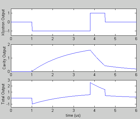
Plot 3: Time evolution of SLED Network Output with a 180 degree drive switch

So what has happened is that we have spent a few microseconds storing up energy in the SLED cavities. That energy radiates out of phase from the direct klystron output. By quickly switching the klystron output after the SLED cavities are filled, the two waves add rather than cancelling, and some "pulse compression" has been performed.

Notice how quickly the SLED output decreases after the 180 degree klystron phase shift. This is because the (new) RF being fed into the SLED cavities opposes the fields already stored. This process is often called 'discharging' the SLED cavities.

Plot 4 below is the absolute value of the combined output from the bottom of plot 3. I have included this picture because it shows basically the structure seen by the SCP "AMPLITUDE FAST TIME PLOT" utility. The amplitude detector which does this measurement (diode recifier) is sensitive to the amplitude of the RF only.

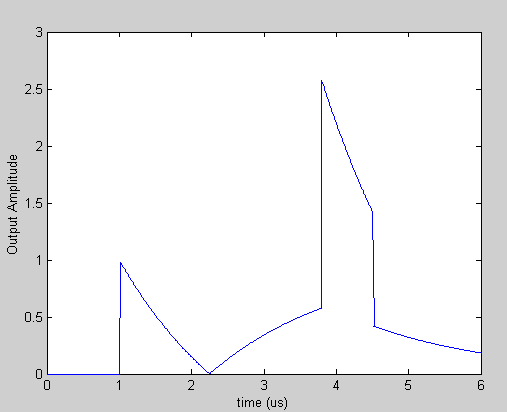
Plot 4: Time Evolution of RF Amplitude of SLED Combined SLED Network

There is one more important part of the story:

So far we have only discussed what SLED does to the klystron output. The other important aspect of this is that we plan to feed this RF into accelerator structures.

Without going into an involved discussion about the transient response of an accelerator structure, we need to recognize the following basic idea: The SLAC standard accelerator has 84 small resonant cavities. As an RF wave is introduced to the first cavity it "fills" (just as in the bottom of plot 1, but with a much shorter time constant), and some of the energy leaks out into the next cell, and so on.

This process also tends to approach an equilibrium condition, and the "fill time constant" for a standard SLAC accelerator is 0.83 uS.

What this structure filling process does is "smear out" (in time) the RF fields available to accelerate a beam. In plot 5 below I show the effect of this structure filling process. Plotted is the SLED output from the bottom of plot 3, "smeared out" by a 0.83 uS filling time constant.

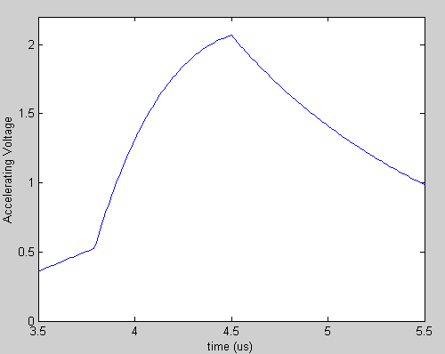
Plot 5: Time Evolution of the Resultant Acceleration Profile

Notice that in plot 5 I have zoomed in (in time) to the most interesting 2 uS portion of this scheme. In this model, the peak acceleration is more than twice that without SLED (but for a very short time).

In the simplistic model used to make these plots, I have ignored the SLED cavity losses completely. In reality the SLED we use has a peak energy multiplication factor of about 1.8 (or so).

Questions for the Reader:

Suppose that just after the time of the switch in phase of the klystron one of the SLED cavities has an internal arc which (instantaneously) collapses all of the energy stored in that cavity. How would this effect the beam acceleration? What other unusual things would happen?

Presume for a moment that the modulator (Pulsed Klystron HVPS) tuning is poor such that there is a large HV ramp across the 5 uS pulse. This causes the klystron output to vary by say 90 degrees (in addition to the 180 degrees shift) uniformly over the RF pulse. How would this effect the acceleration?

Tuning of the SLED cavities is an issue, most importantly since the presumption that the SLED radiated wave is 180 degrees shifted from the prompt klystron wave assumes the cavity resonance is at the same frequency as the driving RF. What happens if both cavities become detuned uniformly? What happens if just one of the cavities becomes detuned?

The Farkas (et. al.) paper referenced points out that if longer RF pulses were available, allowing a longer SLED cavity fill time (by adjusting beta), the energy multiplication factor can be increased. Can you explain why a longer RF pulse and longer SLED fill time would increase the acceleration multiplication factor?